4 Unconstrained Gradient-Based Optimization
In this chapter we focus on unconstrained optimization problems with continuous design variables, which we can write as
where is composed of the design variables that the optimization algorithm can change.
We solve these problems using gradient information to determine a series of steps from a starting guess (or initial design) to the optimum, as shown in Figure 4.1.

Figure 4.1:Gradient-based optimization starts with a guess, , and takes a sequence of steps in -dimensional space that converge to an optimum, .
We assume the objective function to be nonlinear, continuous, and deterministic. We do not assume unimodality or multimodality, and there is no guarantee that the algorithm finds the global optimum. Referring to the attributes that classify an optimization problem (Figure 1.22), the optimization algorithms discussed in this chapter range from first to second order, perform a local search, and evaluate the function directly.
The algorithms are based on mathematical principles rather than heuristics.
Although most engineering design problems are constrained, the constrained optimization algorithms in Chapter 5 build on the methods explained in the current chapter.
4.1 Fundamentals
To determine the step directions shown in Figure 4.1, gradient-based methods need the gradient (first-order information). Some methods also use curvature (second-order information). Gradients and curvature are required to build a second-order Taylor series, a fundamental building block in establishing optimality and developing gradient-based optimization algorithms.
4.1.1 Derivatives and Gradients
Recall that we are considering a scalar objective function , where is the vector of design variables, .
The gradient of this function, , is a column vector of first-order partial derivatives of the function with respect to each design variable:
where each partial derivative is defined as the following limit:
Each component in the gradient vector quantifies the function’s local rate of change with respect to the corresponding design variable, as shown in Figure 4.2 for the two-dimensional case. In other words, these components represent the slope of the function along each coordinate direction. The gradient is a vector pointing in the direction of the greatest function increase from the current point.
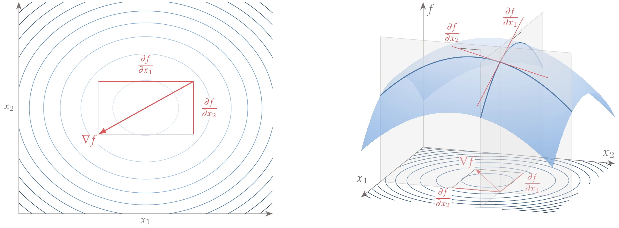
Figure 4.2:Components of the gradient vector in the two-dimensional case.
The gradient vectors are normal to the surfaces of constant in -dimensional space (isosurfaces). In the two-dimensional case, gradient vectors are perpendicular to the function contour lines, as shown in Figure 4.2.[1]
If a function is simple, we can use symbolic differentiation as we did in Example 4.1. However, symbolic differentiation has limited utility for general engineering models because most models are far more complicated; they may include loops, conditionals, nested functions, and implicit equations. Fortunately, there are several methods for computing derivatives numerically; we cover these methods in Chapter 6.
Each gradient component has units that correspond to the units of the function divided by the units of the corresponding variable. Because the variables might represent different physical quantities, each gradient component might have different units.
From an engineering design perspective, it might be helpful to think about relative changes, where the derivative is given as the percentage change in the function for a 1 percent increase in the variable. This relative derivative can be computed by nondimensionalizing both the function and the variable, that is,
where and are the values of the function and variable, respectively, at the point where the derivative is computed.
The gradient components quantify the function’s rate of change in each coordinate direction (), but sometimes we are interested in the rate of change in a direction that is not a coordinate direction. The rate of change in a direction is quantified by a directional derivative, defined as
We can find this derivative by projecting the gradient onto the desired direction using the dot product
When is a unit vector aligned with one of the Cartesian coordinates , this dot product yields the corresponding partial derivative . A two-dimensional example of this projection is shown in Figure 4.5.
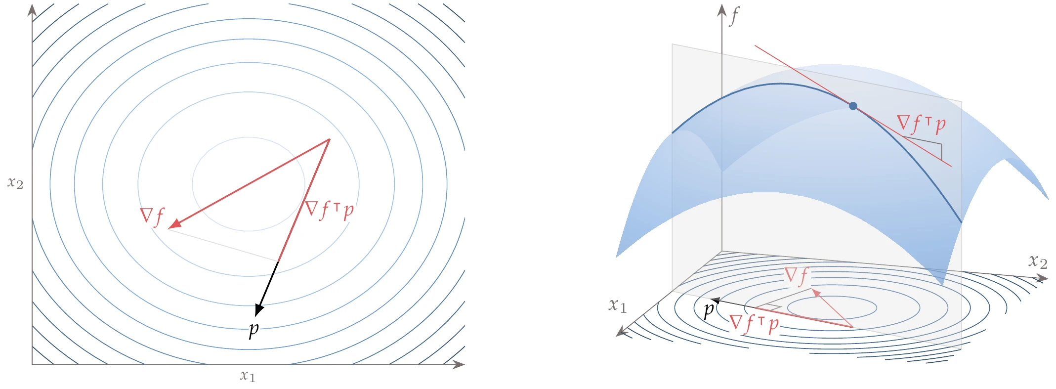
Figure 4.5:Projection of the gradient in an arbitrary unit direction .
From the gradient projection, we can see why the gradient is the direction of the steepest increase. If we use this definition of the dot product,
where is the angle between the two vectors, we can see that this is maximized when . That is, the directional derivative is largest when points in the same direction as .
If is in the interval , the directional derivative is positive and is thus in a direction of increase, as shown in Figure 4.6. If is in the interval , the directional derivative is negative, and points in a descent direction. Finally, if , the directional derivative is 0, and thus the function value does not change for small steps; it is locally flat in that direction. This condition occurs when and are orthogonal; therefore, the gradient is orthogonal to the function isosurfaces.
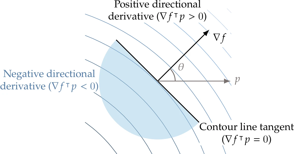
Figure 4.6:The gradient is always orthogonal to contour lines (surfaces), and the directional derivative in the direction is given by .
To get the correct slope in the original units of , the direction should be normalized as . However, in some of the gradient-based algorithms of this chapter, is not normalized because the length contains useful information. If is not normalized, the slopes and variable axis are scaled by a constant.
4.1.2 Curvature and Hessians
The rate of change of the gradient—the curvature—is also useful information because it tells us if a function’s slope is increasing (positive curvature), decreasing (negative curvature), or stationary (zero curvature).
In one dimension, the gradient reduces to a scalar (the slope), and the curvature is also a scalar that can be calculated by taking the second derivative of the function. To quantify curvature in dimensions, we need to take the partial derivative of each gradient component with respect to each coordinate direction , yielding
If the function has continuous second partial derivatives, the order of differentiation does not matter, and the mixed partial derivatives are equal; thus
This property is known as the symmetry of second derivatives or equality of mixed partials.[2]
Considering all gradient components and their derivatives with respect to all coordinate directions results in a second-order tensor. This tensor can be represented as a square matrix of second-order partial derivatives called the Hessian:
The Hessian is expressed in index notation as:
Because of the symmetry of second derivatives, the Hessian is a symmetric matrix with independent elements.
Each row of the Hessian is a vector that quantifies the rate of change of all components of the gradient vector with respect to the direction . On the other hand, each column of the matrix quantifies the rate of change of component of the gradient vector with respect to all coordinate directions . Because the Hessian is symmetric, the rows and columns are transposes of each other, and these two interpretations are equivalent.
We can find the rate of change of the gradient in an arbitrary normalized direction by taking the product . This yields an -vector that quantifies the rate of change of the gradient in the direction , where each component of the vector is the rate of the change of the corresponding partial derivative with respect to a movement along . Therefore, this product is defined as follows:
Because of the symmetry of second derivatives, we can also interpret this as the rate of change in the directional derivative of the function along with respect to each of the components of .
To find the curvature of the one-dimensional function along a direction , we need to project onto direction as
which yields a scalar quantity. Again, if we want to get the curvature in the original units of , should be normalized.
For an -dimensional Hessian, it is possible to find directions (where ) along which the projected curvature aligns with that direction, that is,
This is an eigenvalue problem whose eigenvectors represent the principal curvature directions, and the eigenvalues quantify the corresponding curvatures. If each eigenvector is normalized as , then the corresponding is the curvature in the original units.
4.1.3 Taylor Series
The Taylor series provides a local approximation to a function and is the foundation for gradient-based optimization algorithms.
For an -dimensional function, the Taylor series can predict the function along any direction . This is done by projecting the gradient and Hessian onto the desired direction to get an approximation of the function at any nearby point :[3]
We use a second-order Taylor series (ignoring the cubic term) because it results in a quadratic, the lowest-order Taylor series that can have a minimum. For a function that is continuous, this approximation can be made arbitrarily accurate by making small enough.
4.1.4 Optimality Conditions
To find the minimum of a function, we must determine the mathematical conditions that identify a given point as a minimum. There is only a limited set of problems for which we can prove global optimality, so in general, we are only interested in local optimality.
A point is a local minimum if for all in the neighborhood of . In other words, there must be no descent direction starting from the local minimum.
A second-order Taylor series expansion about for small steps of size yields
For to be an optimal point, we must have for all . This implies that the first- and second-order terms in the Taylor series have to be nonnegative, that is,
Because the magnitude of is small, we can always find a such that the first term dominates. Therefore, we require that
Because can be in any arbitrary direction, the only way this inequality can be satisfied is if all the elements of the gradient are zero (refer to Figure 4.6),
This is the first-order necessary optimality condition for an unconstrained problem. This is necessary because if any element of is nonzero, there are descent directions (e.g., ) for which the inequality would not be satisfied.
Because the gradient term has to be zero, we must now satisfy the remaining term in the inequality (Equation 4.17), that is,
From Equation 4.13, we know that this term represents the curvature in direction , so this means that the function curvature must be positive or zero when projected in any direction. You may recognize this inequality as the definition of a positive-semidefinite matrix. In other words, the Hessian must be positive semidefinite.
For a matrix to be positive semidefinite, its eigenvalues must all be greater than or equal to zero. Recall that the eigenvalues of the Hessian quantify the principal curvatures, so as long as all the principal curvatures are greater than or equal to zero, the curvature along an arbitrary direction is also greater than or equal to zero.
These conditions on the gradient and curvature are necessary conditions for a local minimum but are not sufficient. They are not sufficient because if the curvature is zero in some direction (i.e., ), we have no way of knowing if it is a minimum unless we check the third-order term. In that case, even if it is a minimum, it is a weak minimum.
The sufficient conditions for optimality require the curvature to be positive in any direction, in which case we have a strong minimum.
Mathematically, this means that for all nonzero , which is the definition of a positive-definite matrix.
If is a positive-definite matrix, every eigenvalue of is positive.[4]Figure 4.11 shows some examples of quadratic functions that are positive definite (all positive eigenvalues), positive semidefinite (nonnegative eigenvalues), indefinite (mixed eigenvalues), and negative definite (all negative eigenvalues).
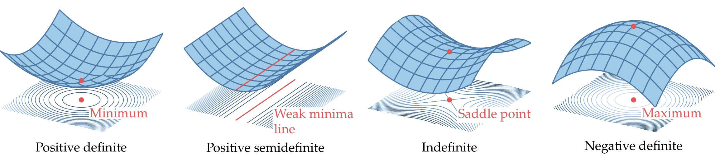
Figure 4.11:Quadratic functions with different types of Hessians.
In summary, the necessary optimality conditions for an unconstrained optimization problem are
The sufficient optimality conditions are
We may be able to solve the optimality conditions analytically for simple problems, as we did in Example 4.7. However, this is not possible in general because the resulting equations might not be solvable in closed form. Therefore, we need numerical methods that solve for these conditions.
When using a numerical approach, we seek points where , but the entries in do not converge to exactly zero because of finite-precision arithmetic. Instead, we define convergence for the first criterion based on the maximum component of the gradient, such that
where is some tolerance. A typical absolute tolerance is or a six-order magnitude reduction in gradient when using a relative tolerance. Absolute and relative criteria are often combined in a metric such as the following:
where is the gradient at the starting point.
The second optimality condition (that must be positive semidefinite) is not usually checked explicitly. If we satisfy the first condition, then all we know is that we have reached a stationary point, which could be a maximum, a minimum, or a saddle point. However, as shown in Section 4.4, the search directions for the algorithms of this chapter are always descent directions, and therefore in practice, they should converge to a local minimum.
For a practical algorithm, other exit conditions are often used besides the reduction in the norm of the gradient. A function might be poorly scaled, be noisy, or have other numerical issues that prevent it from ever satisfying this optimality condition (Equation 4.24). To prevent the algorithm from running indefinitely, it is common to set a limit on the computational budget, such as the number of function calls, the number of major iterations, or the clock time. Additionally, to detect a case where the optimizer is not making significant progress and not likely to improve much further, we might set criteria on the minimum step size and the minimum change in the objective. Similar to the conditions on the gradient, the minimum change in step size could be limited as follows:
The absolute and relative conditions on the objective are of the same form, although they only use an absolute value rather than a norm because the objective is scalar.
4.2 Two Overall Approaches to Finding an Optimum
Although the optimality conditions derived in the previous section can be solved analytically to find the function minima, this analytic approach is not possible for functions that result from numerical models. Instead, we need iterative numerical methods to find minima based only on the function values and gradients.
In Chapter 3, we reviewed methods for solving simultaneous systems of nonlinear equations, which we wrote as . Because the first-order optimality condition () can be written in this residual form (where and ), we could try to use the solvers from Chapter 3 directly to solve unconstrained optimization problems. Although several components of general solvers for are used in optimization algorithms, these solvers are not the most effective approaches in their original form. Furthermore, solving is not necessarily sufficient—it finds a stationary point but not necessarily a minimum. Optimization algorithms require additional considerations to ensure convergence to a minimum.
Like the iterative solvers from Chapter 3, gradient-based algorithms start with a guess, , and generate a series of points, that converge to a local optimum, , as previously illustrated in Figure 4.1. At each iteration, some form of the Taylor series about the current point is used to find the next point.
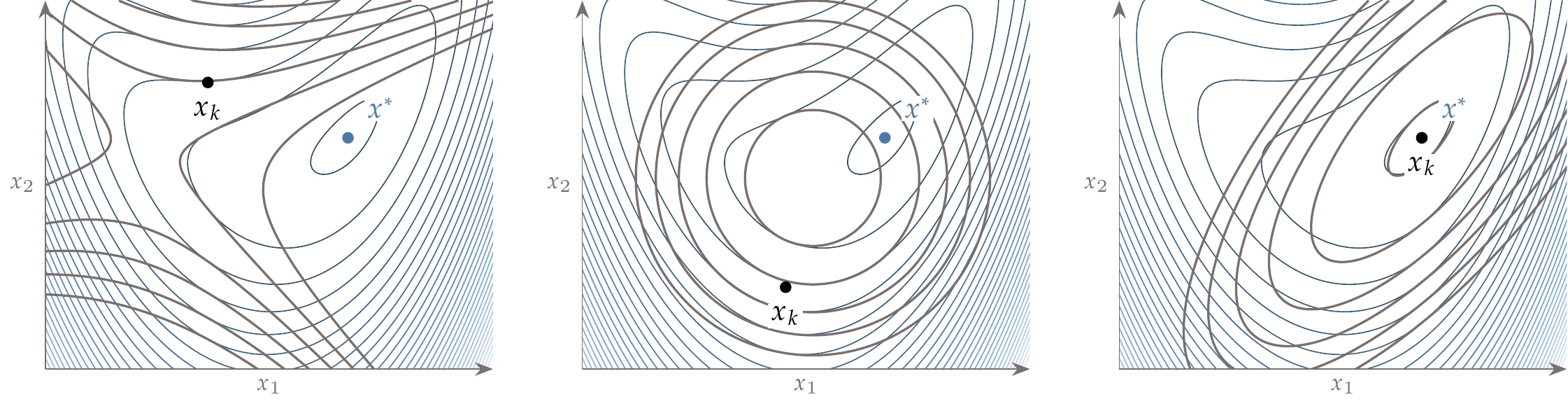
Figure 4.13:Taylor series quadratic models are only guaranteed to be accurate near the point about which the series is expanded ().
A truncated Taylor series is, in general, only a good model within a small neighborhood, as shown in Figure 4.13, which shows three quadratic models of the same function based on three different points.
All quadratic approximations match the local gradient and curvature at the respective points. However, the Taylor series quadratic about the first point (left plot) yields a quadratic without a minimum (the only critical point is a saddle point). The second point (middle plot) yields a quadratic whose minimum is closer to the true minimum. Finally, the Taylor series about the actual minimum point (right plot) yields a quadratic with the same minimum, as expected, but we can see how the quadratic model worsens the farther we are from the point.
Because the Taylor series is only guaranteed to be a good model locally, we need a globalization strategy to ensure convergence to an optimum. Globalization here means making the algorithm robust enough that it can converge to a local minimum when starting from any point in the domain. This should not be confused with finding the global minimum, which is a separate issue (see Tip 4.8). There are two main globalization strategies: line search and trust region.
The line search approach consists of three main steps for every iteration (Figure 4.14):
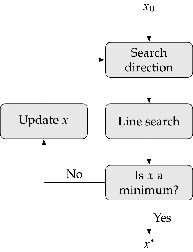
Figure 4.14:Line search approach.
Choose a suitable search direction from the current point. The choice of search direction is based on a Taylor series approximation.
Determine how far to move in that direction by performing a line search.
Move to the new point and update all values.
The two first steps can be seen as two separate subproblems. We address the line search subproblem in Section 4.3 and the search direction subproblem in Section 4.4.
Trust-region methods also consist of three steps (Figure 4.15):
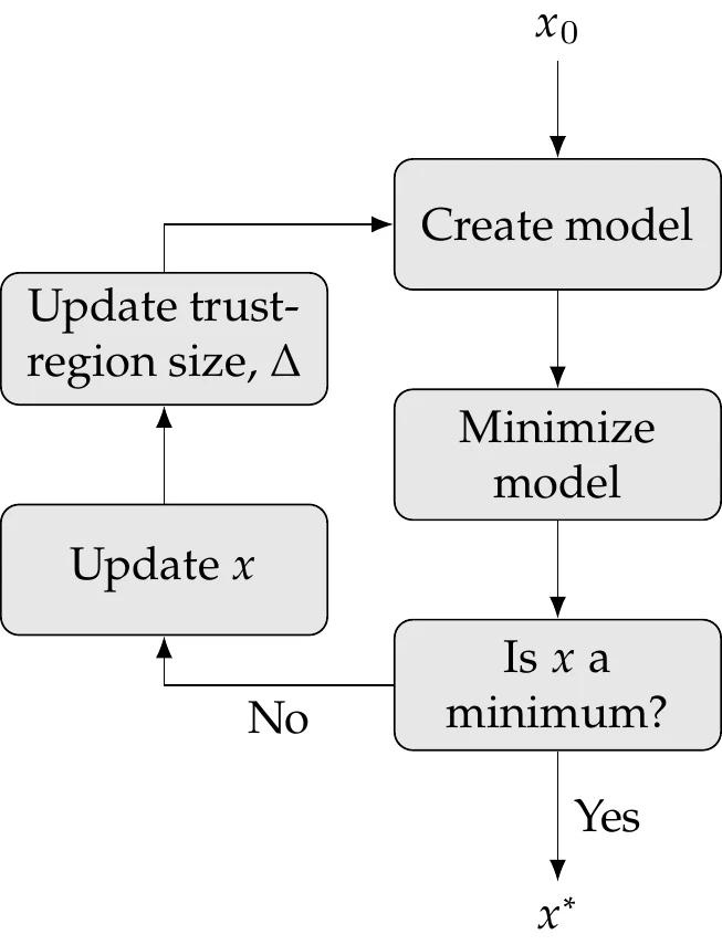
Figure 4.15:Trust-region approach.
Create a model about the current point. This model can be based on a Taylor series approximation or another type of surrogate model.
Minimize the model within a trust region around the current point to find the step.
Move to the new point, update values, and adapt the size of the trust region.
We introduce the trust-region approach in Section 4.5. However, we devote more attention to algorithms that use the line search approach because they are more common in general nonlinear optimization.
Both line search and trust-region approaches use iterative processes that must be repeated until some convergence criterion is satisfied. The first step in both approaches is usually referred to as a major iteration, whereas the second step might require more function evaluations corresponding to minor iterations.
4.3 Line Search
Gradient-based unconstrained optimization algorithms that use a line search follow Algorithm 4.1. We start with a guess and provide a convergence tolerance for the optimality condition.[5]The final output is an optimal point and the corresponding function value . As mentioned in the previous section, there are two main subproblems in line search gradient-based optimization algorithms: choosing the search direction and determining how far to step in that direction. In the next section, we introduce several methods for choosing the search direction. The line search method determines how far to step in the chosen direction and is usually independent of the method for choosing the search direction. Therefore, line search methods can be combined with any method for finding the search direction. However, the search direction method determines the name of the overall optimization algorithm, as we will see in the next section.
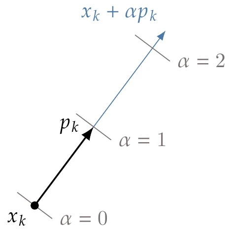
Figure 4.16:The line search starts from a given point and searches solely along direction .
For the line search subproblem, we assume that we are given a starting location at and a suitable search direction along which to search (Figure 4.16). The line search then operates solely on points along direction starting from , which can be written as
where the scalar is always positive and represents how far we go in the direction . This equation produces a one-dimensional slice of -dimensional space, as illustrated in Figure 4.17.
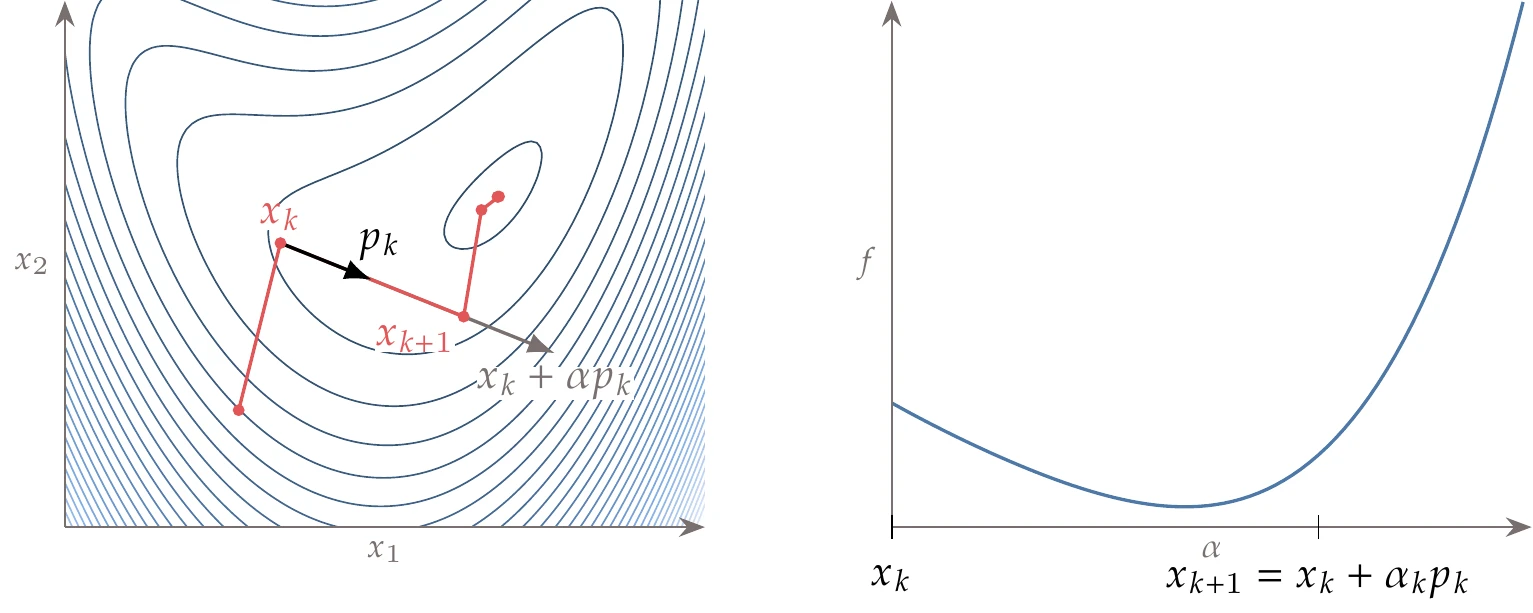
Figure 4.17:The line search projects the -dimensional problem onto one dimension, where the independent variable is .
The line search determines the magnitude of the scalar , which in turn determines the next point in the iteration sequence. Even though and are -dimensional, the line search is a one-dimensional problem with the goal of selecting .
Line search methods require that the search direction be a descent direction so that (see Figure 4.18). This guarantees that can be reduced by stepping some distance along this direction with a positive .
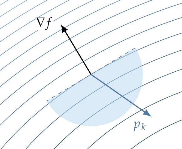
Figure 4.18:The line search direction must be a descent direction.
The goal of the line search is not to find the value of that minimizes but to find a point that is “good enough” using as few function evaluations as possible. This is because finding the exact minimum along the line would require too many evaluations of the objective function and possibly its gradient. Because the overall optimization needs to find a point in -dimensional space, the search direction might change drastically between line searches, so spending too many iterations on each line search is generally not worthwhile.
Consider the bean function whose contours are shown in Figure 4.19.
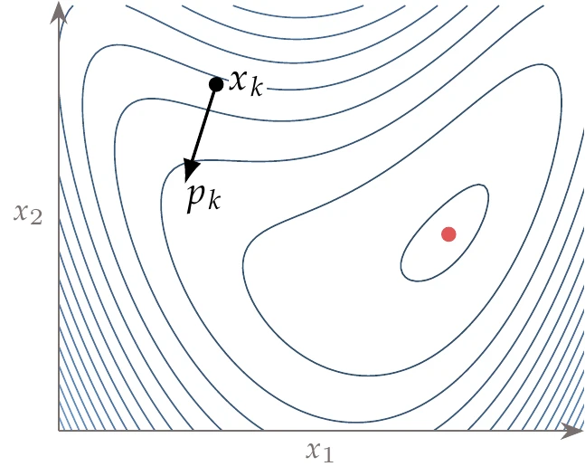
Figure 4.19:The descent direction does not necessarily point toward the minimum, in which case it would be wasteful to do an exact line search.
At point , the direction is a descent direction. However, it would be wasteful to spend a lot of effort determining the exact minimum in the direction because it would not take us any closer to the minimum of the overall function (the dot on the right side of the plot). Instead, we should find a point that is good enough and then update the search direction.
To simplify the notation for the line search, we define the single-variable function
where corresponds to the start of the line search ( in Figure 4.17), and thus . Then, using , the slope of the single-variable function is
Substituting into the derivatives results in
which is the directional derivative along the search direction. The slope at the start of a given line search is
Because must be a descent direction, is always negative. Figure 4.20 is a version of the one-dimensional slice from Figure 4.17 in this notation. The axis and the slopes scale with the magnitude of .
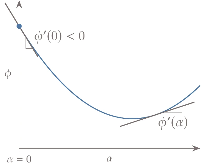
Figure 4.20:For the line search, we denote the function as with the same value as . The slope is the gradient of projected onto the search direction.
4.3.1 Sufficient Decrease and Backtracking
The simplest line search algorithm to find a “good enough” point relies on the sufficient decrease condition combined with a backtracking algorithm. The sufficient decrease condition, also known as the Armijo condition, is given by the inequality
where is a constant such that .[6] The quantity represents the expected decrease of the function, assuming the function continued at the same slope. The multiplier states that Equation 4.31 will be satisfied as long we achieve even a small fraction of the expected decrease, as shown in Figure 4.21.
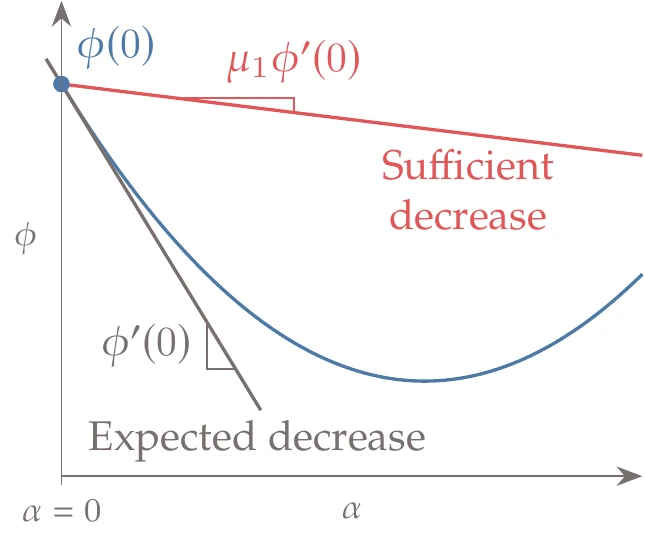
Figure 4.21:The sufficient decrease line has a slope that is a small fraction of the slope at the start of the line search.
In practice, this constant is several orders of magnitude smaller than 1, typically .
Because is a descent direction, and thus , there is always a positive that satisfies this condition for a smooth function.
The concept is illustrated in Figure 4.22, which shows a function with a negative slope at and a sufficient decrease line whose slope is a fraction of that initial slope. When starting a line search, we know the function value and slope at , so we do not really know how the function varies until we evaluate it. Because we do not want to evaluate the function too many times, the first point whose value is below the sufficient decrease line is deemed acceptable. The sufficient decrease line slope in Figure 4.22 is exaggerated for illustration purposes; for typical values of , the line is indistinguishable from horizontal when plotted.
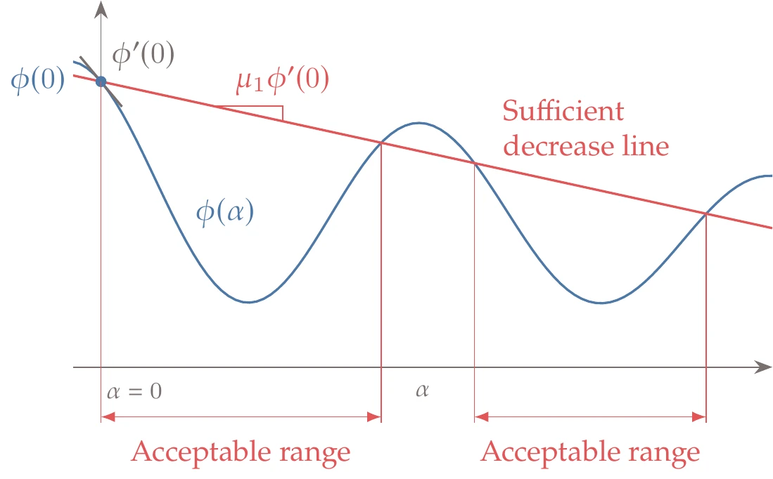
Figure 4.22:Sufficient decrease condition.
Line search algorithms require a first guess for . As we will see later, some methods for finding the search direction also provide good guesses for the step length. However, in many cases, we have no idea of the scale of function, so our initial guess may not be suitable. Even if we do have an educated guess for , it is only a guess, and the first step might not satisfy the sufficient decrease condition.
A straightforward algorithm that is guaranteed to find a step that satisfies the sufficient decrease condition is backtracking (Algorithm 4.2). This algorithm starts with a maximum step and successively reduces the step by a constant ratio until it satisfies the sufficient decrease condition (a typical value is ). Because the search direction is a descent direction, we know that we will achieve an acceptable decrease in function value if we backtrack enough.
Although backtracking is guaranteed to find a point that satisfies sufficient decrease, there are two undesirable scenarios where this algorithm performs poorly. The first scenario is that the guess for the initial step is far too large, and the step sizes that satisfy sufficient decrease are smaller than the starting step by several orders of magnitude. Depending on the value of , this scenario requires a large number of backtracking evaluations.
The other undesirable scenario is where our initial guess immediately satisfies sufficient decrease. However, the function’s slope is still highly negative, and we could have decreased the function value by much more if we had taken a larger step. In this case, our guess for the initial step is far too small.
Even if our original step size is not too far from an acceptable step size, the basic backtracking algorithm ignores any information we have about the function values and gradients. It blindly takes a reduced step based on a preselected ratio . We can make more intelligent estimates of where an acceptable step is based on the evaluated function values (and gradients, if available). The next section introduces a more sophisticated line search algorithm that deals with these scenarios much more efficiently.
4.3.2 Strong Wolfe Conditions
One major weakness of the sufficient decrease condition is that it accepts small steps that marginally decrease the objective function because in Equation 4.31 is typically small. We could increase (i.e., tilt the red line downward in Figure 4.22) to prevent these small steps; however, that would prevent us from taking large steps that still result in a reasonable decrease. A large step that provides a reasonable decrease is desirable because large steps generally lead to faster convergence. Therefore, we want to prevent overly small steps while not making it more difficult to accept reasonable large steps. We can accomplish this by adding a second condition to construct a more efficient line search algorithm.
Just like guessing the step size, it is difficult to know in advance how much of a function value decrease to expect. However, if we compare the slope of the function at the candidate point with the slope at the start of the line search, we can get an idea if the function is “bottoming out”, or flattening, using the sufficient curvature condition:
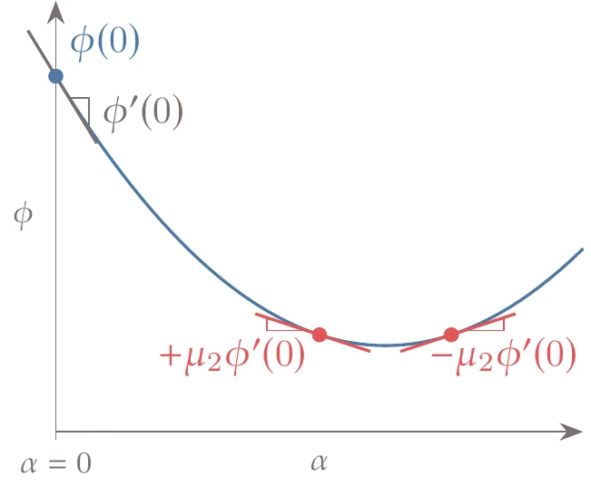
Figure 4.25:The sufficient curvature condition requires the function slope magnitude to be a fraction of the initial slope.
This condition requires that the magnitude of the slope at the new point be lower than the magnitude of the slope at the start of the line search by a factor of , as shown in Figure 4.25. This requirement is called the sufficient curvature condition because by comparing the two slopes, we quantify the function’s rate of change in the slope—the curvature. Typical values of range from 0.1 to 0.9, and the best value depends on the method for determining the search direction and is also problem dependent.
As tends to zero, enforcing the sufficient curvature condition tends toward a point where , which would yield an exact line search.
The sign of the slope at a point satisfying this condition is not relevant; all that matters is that the function slope be shallow enough. The idea is that if the slope is still negative with a magnitude similar to the slope at the start of the line search, then the step is too small, and we expect the function to decrease even further by taking a larger step. If the slope is positive with a magnitude similar to that at the start of the line search, then the step is too large, and we expect to decrease the function further by taking a smaller step. On the other hand, when the slope is shallow enough (either positive or negative), we assume that the candidate point is near a local minimum, and additional effort yields only incremental benefits that are wasteful in the context of the larger problem.
The sufficient decrease and sufficient curvature conditions are collectively known as the strong Wolfe conditions. Figure 4.26 shows acceptable intervals that satisfy the strong Wolfe conditions, which are more restrictive than the sufficient decrease condition (Figure 4.22).
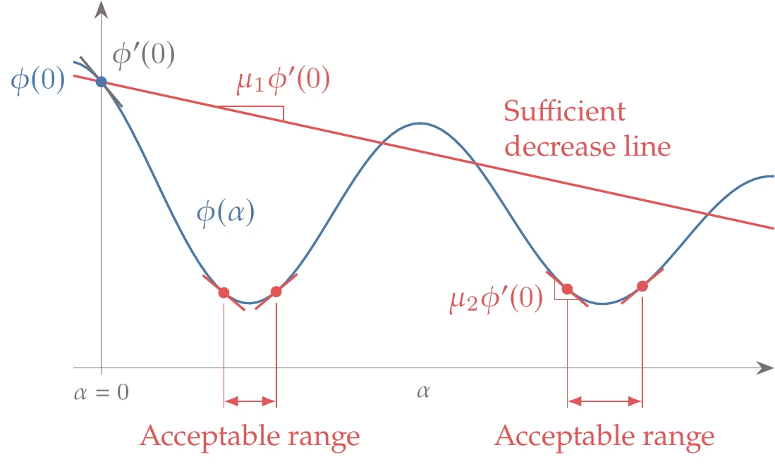
Figure 4.26:Steps that satisfy the strong Wolfe conditions.
The sufficient decrease slope must be shallower than the sufficient curvature slope, that is, . This is to guarantee that there are steps that satisfy both the sufficient decrease and sufficient curvature conditions. Otherwise, the situation illustrated in Figure 4.27 could take place.
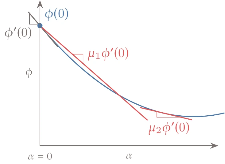
Figure 4.27:If , there might be no point that satisfies the strong Wolfe conditions.
We now present a line search algorithm that finds a step satisfying the strong Wolfe conditions. Enforcing the sufficient curvature condition means we require derivative information (), at least using the derivative at the beginning of the line search that we already computed from the gradient. There are various line search algorithms in the literature, including some that are derivative-free.
Here, we detail a line search algorithm based on the one developed by Moré and Thuente.3[7]
The algorithm has two phases:
The bracketing phase finds an interval within which we are certain to find a point that satisfies the strong Wolfe conditions.
The pinpointing phase finds a point that satisfies the strong Wolfe conditions within the interval provided by the bracketing phase.
The bracketing phase is given by Algorithm 4.3 and illustrated in Figure 4.28. For brevity, we use a notation in the following algorithms where, for example, and . Overall, the bracketing algorithm increases the step size until it either finds an interval that must contain a point satisfying the strong Wolfe conditions or a point that already meets those conditions.
We start the line search with a guess for the step size, which defines the first interval. For a smooth continuous function, we are guaranteed to have a minimum within an interval if either of the following hold:
The function value at the candidate step is higher than the value at the start of the line search.
The step satisfies sufficient decrease, and the slope is positive.
These two scenarios are illustrated in the top two rows of Figure 4.28. In either case, we have an interval within which we can find a point that satisfies the strong Wolfe conditions using the pinpointing algorithm. The order in arguments to the pinpoint function in Algorithm 4.3 is significant because this function assumes that the function value corresponding to the first is the lower one.
The third row in Figure 4.28 illustrates the scenario where the point satisfies the strong Wolfe conditions, in which case the line search is finished.
If the point satisfies sufficient decrease and the slope at that point is negative, we assume that there are better points farther along the line, and the algorithm increases the step size. This larger step and the previous one define a new interval that has moved away from the line search starting point. We repeat the procedure and check the scenarios for this new interval. To save function calls, bracketing should return not just but also the corresponding function value and gradient to the outer function.
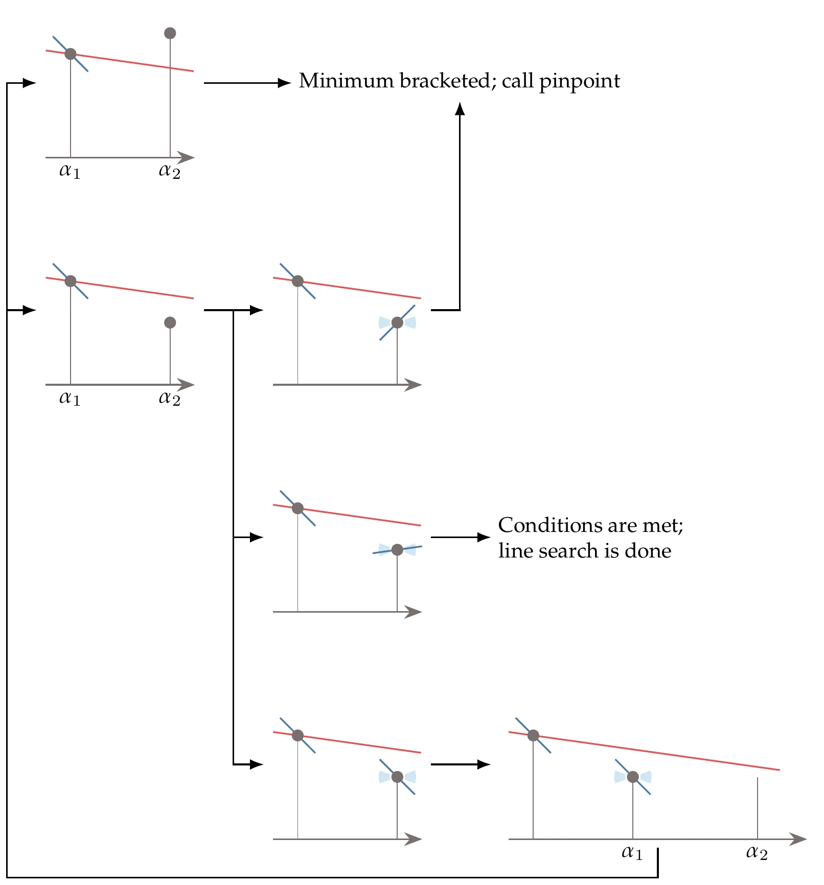
Figure 4.28:Visual representation of the bracketing algorithm. The sufficient decrease line is drawn as if were the starting point for the line search, which is the case for the first line search iteration but not necessarily the case for later iterations.
If the bracketing phase does not find a point that satisfies the strong Wolfe conditions, it finds an interval where we are guaranteed to find such a point in the pinpointing phase described in Algorithm 4.4 and illustrated in Figure 4.29. The intervals generated by this algorithm, bounded by and , always have the following properties:
The interval has one or more points that satisfy the strong Wolfe conditions.
Among all the points generated so far that satisfy the sufficient decrease condition, has the lowest function value.
The slope at decreases toward .
The first step of pinpointing is to find a new point within the given interval. Various techniques can be used to find such a point. The simplest one is to select the midpoint of the interval (bisection), but this method is limited to a linear convergence rate. It is more efficient to perform interpolation and select the point that minimizes the interpolation function, which can be done analytically (see Section 4.3.3). Using this approach, we can achieve quadratic convergence.
Once we have a new point within the interval, four scenarios are possible, as shown in Figure 4.29. The first scenario is that is above the sufficient decrease line or greater than or equal to . In that scenario, becomes the new , and we have a new smaller interval.
In the second, third, and fourth scenarios, is below the sufficient decrease line, and . In those scenarios, we check the value of the slope . In the second and third scenarios, we choose the new interval based on the direction in which the slope predicts a local decrease. If the slope is shallow enough (fourth scenario), we have found a point that satisfies the strong Wolfe conditions.
In theory, the line search given in Algorithm 4.3 followed by Algorithm 4.4 is guaranteed to find a step length satisfying the strong Wolfe conditions. In practice, some additional considerations are needed for improved robustness. One of these criteria is to ensure that the new point in the pinpoint algorithm is not so close to an endpoint as to cause the interpolation to be ill-conditioned. A fallback option in case the interpolation fails could be a simpler algorithm, such as bisection. Another criterion is to ensure that the loop does not continue indefinitely in case finite-precision arithmetic leads to indistinguishable function value changes. A limit on the number of iterations might be necessary.
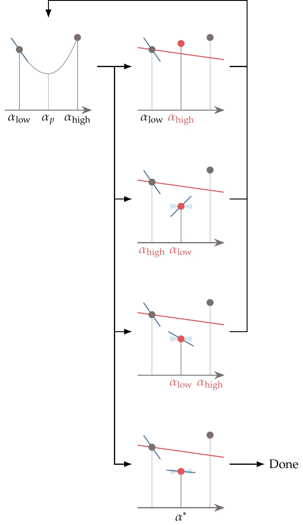
Figure 4.29:Visual representation of the pinpointing algorithm. The labels in red indicate the new interval endpoints.
4.3.3 Interpolation for Pinpointing
Interpolation is recommended to find a new point within each interval at the pinpointing phase. Once we have an interpolation function, we find the new point by determining the analytic minimum of that function. This accelerates the convergence compared with bisection. We consider two options: quadratic interpolation and cubic interpolation.
Because we have the function value and derivative at one endpoint of the interval and at least the function value at the other endpoint, one option is to perform quadratic interpolation to estimate the minimum within the interval.
The quadratic can be written as
where , , and are constants to be determined by interpolation. Suppose that we have the function value and the derivative at and the function value at , as illustrated in Figure 4.31. These values correspond to and in the pinpointing algorithm, but we use the more generic indices 1 and 2 because the formulas of this section are not dependent on which one is lower or higher. Then, the boundary conditions at the endpoints are
We can use these three equations to find the three coefficients based on function and derivative values. Once we have the coefficients for the quadratic, we can find the minimum of the quadratic analytically by finding the point such that , which is . Substituting the analytic solution for the coefficients as a function of the given values into this expression yields the final expression for the minimizer of the quadratic:
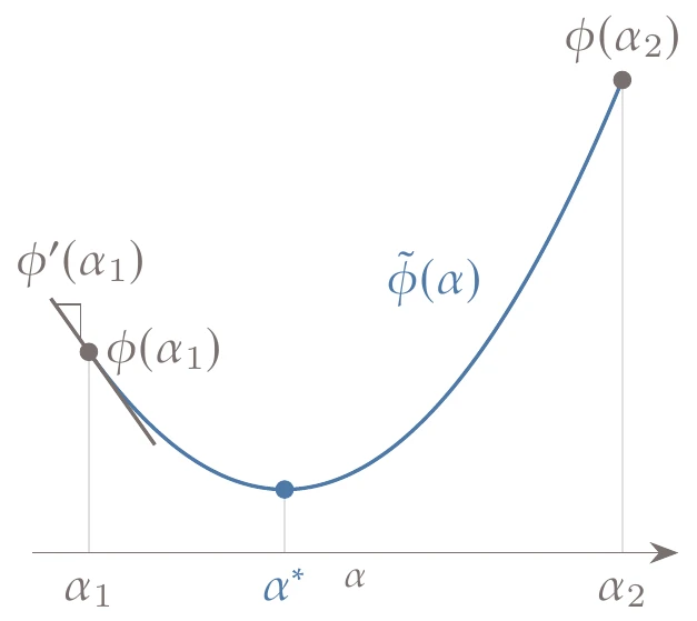
Figure 4.31:Quadratic interpolation with two function values and one derivative.
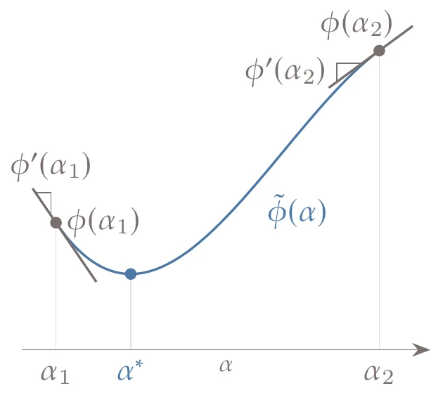
Figure 4.32:Cubic interpolation with function values and derivatives at endpoints.
Performing this quadratic interpolation for successive intervals is similar to the Newton method and also converges quadratically. The pure Newton method also models a quadratic, but it is based on the information at a single point (function value, derivative, and curvature), as opposed to information at two points.
If computing additional derivatives is inexpensive, or we already evaluated (either as part of Algorithm 4.3 or as part of checking the strong Wolfe conditions in Algorithm 4.4), then we have the function values and derivatives at both points. With these four pieces of information, we can perform a cubic interpolation,
as shown in Figure 4.32. To determine the four coefficients, we apply the boundary conditions:
Using these four equations, we can find expressions for the four coefficients as a function of the four pieces of information. Similar to the quadratic interpolation function, we can find the solution for as a function of the coefficients.
There could be two valid solutions, but we are only interested in the minimum, for which the curvature is positive; that is, .
Substituting the coefficients with the expressions obtained from solving the boundary condition equations and selecting the minimum solution yields
where
These interpolations become ill-conditioned if the interval becomes too small. The interpolation may also lead to points outside the bracket. In such cases, we can switch to bisection for the problematic iterations.
4.4 Search Direction
As stated at the beginning of this chapter, each iteration of an unconstrained gradient-based algorithm consists of two main steps: determining the search direction and performing the line search (Algorithm 4.1). The optimization algorithms are named after the method used to find the search direction, , and can use any suitable line search. We start by introducing two first-order methods that only require the gradient and then explain two second-order methods that require the Hessian, or at least an approximation of the Hessian.
4.4.1 Steepest Descent
The steepest-descent method (also called gradient descent) is a simple and intuitive method for determining the search direction. As discussed in Section 4.1.1, the gradient points in the direction of steepest increase, so points in the direction of steepest descent, as shown in Figure 4.33. Thus, our search direction at iteration is simply
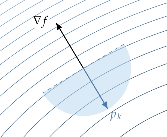
Figure 4.33:The steepest-descent direction points in the opposite direction of the gradient.
One major issue with the steepest descent is that, in general, the entries in the gradient and its overall scale can vary greatly depending on the magnitudes of the objective function and design variables. The gradient itself contains no information about an appropriate step length, and therefore the search direction is often better posed as a normalized direction,
Algorithm 4.5 provides the complete steepest descent procedure.
Regardless of whether we choose to normalize the search direction or not, the gradient does not provide enough information to inform a good guess of the initial step size for the line search. As we saw in Section 4.3, this initial choice has a large impact on the efficiency of the line search because the first guess could be orders of magnitude too small or too large. The second-order methods described later in this section are better in this respect. In the meantime, we can make a guess of the step size for a given line search based on the result of the previous one. Assuming that we will obtain a decrease in objective function at the current line search that is comparable to the previous one, we can write
Solving for the step length, we obtain the guess
Although this expression could be simplified for the steepest descent, we leave it as is so that it is applicable to other methods.
If the slope of the function increases in magnitude relative to the previous line search, this guess decreases relative to the previous line search step length, and vice versa. This is just the first step length in the new line search, after which we proceed as usual.
Although steepest descent sounds like the best possible search direction for decreasing a function, it generally is not. The reason is that when a function curvature varies significantly with direction, the gradient alone is a poor representation of function behavior beyond a small neighborhood, as illustrated previously in Figure 4.19.
The behavior shown in Example 4.10 is expected, and we can show it mathematically. Assuming we perform an exact line search at each iteration, this means selecting the optimal value for along the line search:
Hence, each search direction is orthogonal to the previous one. When performing an exact line search, the gradient projection in the line search direction vanishes at the minimum, which means that the gradient is orthogonal to the search direction, as shown in Figure 4.35.
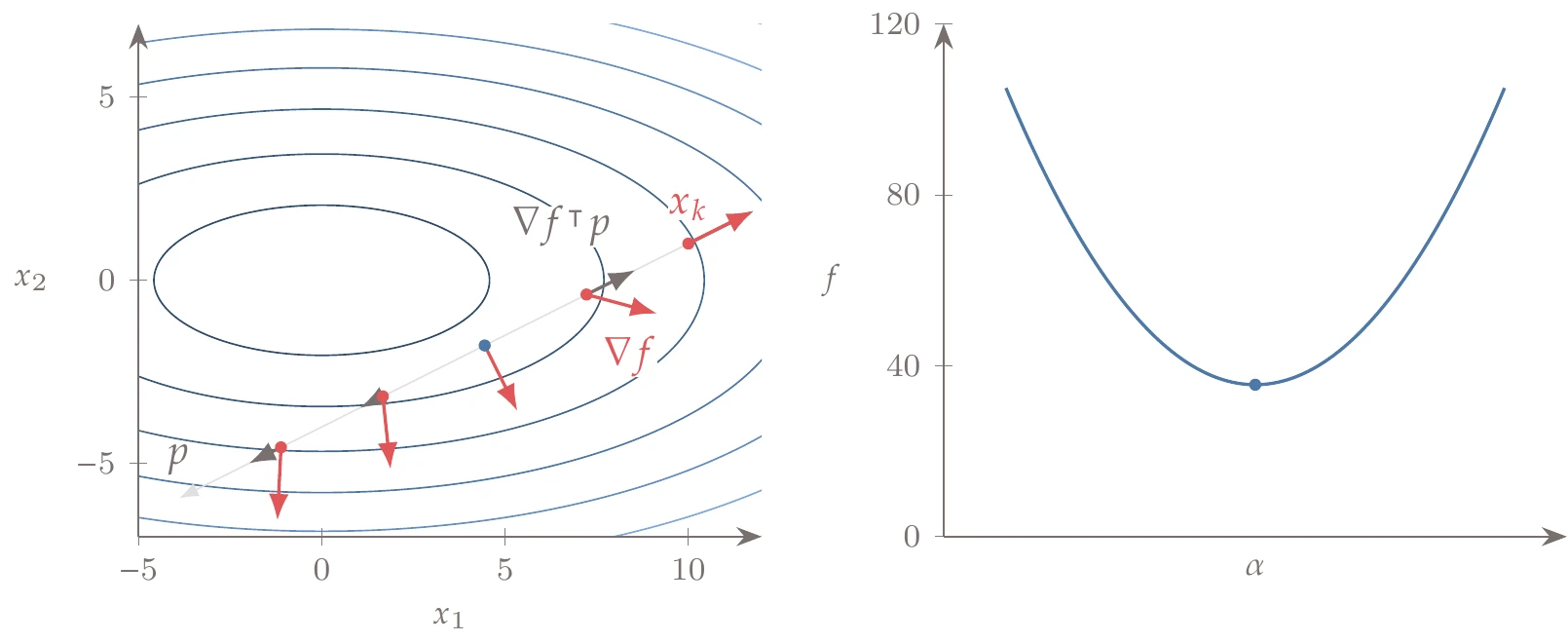
Figure 4.35:The gradient projection in the line search direction vanishes at the line search minimum.
As discussed in the last section, exact line searches are not desirable, so the search directions are not orthogonal. However, the overall zigzagging behavior still exists.
4.4.2 Conjugate Gradient
Steepest descent generally performs poorly, especially if the problem is not well scaled, like the quadratic example in Figure 4.34. The conjugate gradient method updates the search directions such that they do not zigzag as much. This method is based on the linear conjugate gradient method, which was designed to solve linear equations. We first introduce the linear conjugate gradient method and then adapt it to the nonlinear case.
For the moment, let us assume that we have the following quadratic objective function:
where is a positive definite Hessian, and is the gradient at . The constant term is omitted with no loss of generality because it does not change the location of the minimum. To find the minimum of this quadratic, we require
Thus, finding the minimum of a quadratic amounts to solving the linear system , and the residual vector is the gradient of the quadratic.
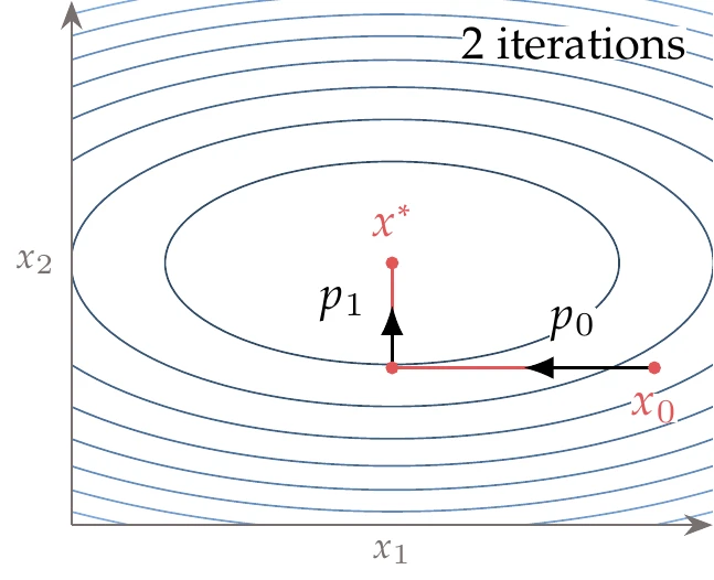
Figure 4.38:For a quadratic function with elliptical contours and the principal axis aligned with the coordinate axis, we can find the minimum in steps, where is the number of dimensions, by using a coordinate search.
If were a positive-definite diagonal matrix, the contours would be elliptical, as shown in Figure 4.38 (or hyper-ellipsoids in the -dimensional case), and the axes of the ellipses would align with the coordinate directions. In that case, we could converge to the minimum by successively performing an exact line search in each coordinate direction for a total of line searches.
In the more general case (but still assuming to be positive definite), the axes of the ellipses form an orthogonal coordinate system in some other orientation. A coordinate search would no longer work as well in this case, as illustrated in Figure 4.39.
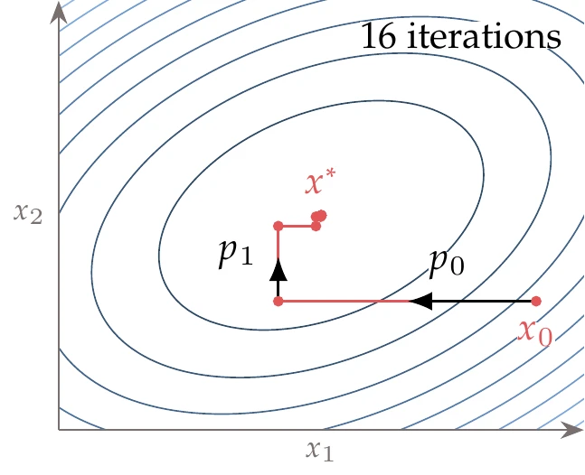
Figure 4.39:For a quadratic function with the elliptical principal axis not aligned with the coordinate axis, more iterations are needed to find the minimum using a coordinate search.
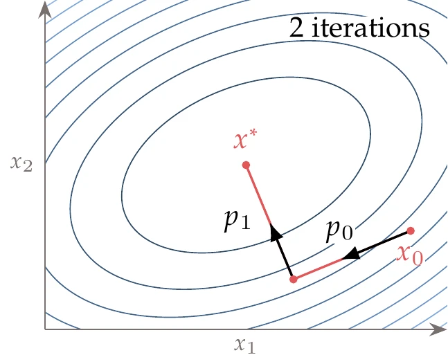
Figure 4.40:We can converge to the minimum of a quadratic function by minimizing along each Hessian eigenvector.
Recall from Section 4.1.2 that the eigenvectors of the Hessian represent the directions of principal curvature, which correspond to the axes of the ellipses. Therefore, we could successively perform a line search along the direction defined by each eigenvector and again converge to the minimum with line searches, as illustrated in Figure 4.40. The problem with this approach is that we would have to compute the eigenvectors of , a computation whose cost is .
Fortunately, the eigenvector directions are not the only set of directions that can minimize the quadratic function in line searches. To find out which directions can achieve this, let us express the path from the origin to the minimum of the quadratic as a sequence of steps with directions and length ,
Thus, we have represented the solution as a linear combination of vectors. Substituting this into the quadratic (Equation 4.48), we get
Suppose that the vectors are conjugate with respect to ; that is, they have the following property:
Then, the double-sum term in Equation 4.51 can be simplified to a single sum and we can write
Because each term in this sum involves only one direction , we have reduced the original problem to a series of one-dimensional quadratic functions that can be minimized one at a time. Two possible conjugate directions are shown for the two-dimensional case in Figure 4.41.
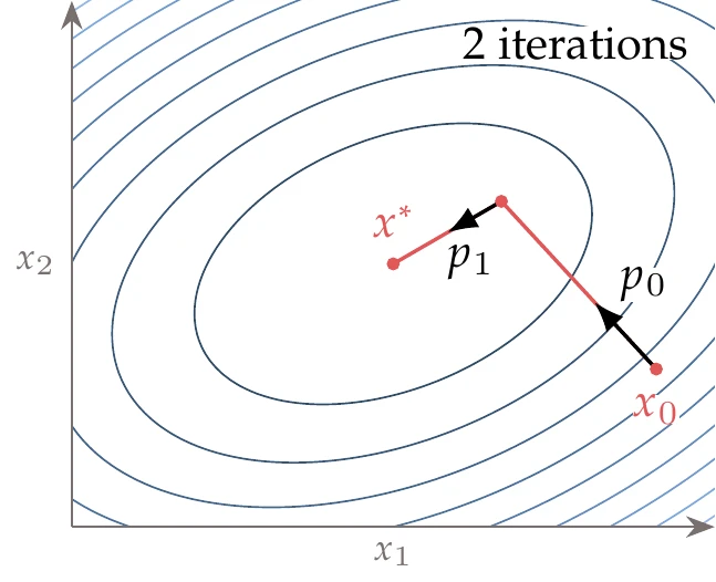
Figure 4.41:By minimizing along a sequence of conjugate directions in turn, we can find the minimum of a quadratic in steps, where is the number of dimensions.
Each one-dimensional problem corresponds to minimizing the quadratic with respect to the step length . Differentiating each term and setting it to zero yields
which corresponds to the result of an exact line search in direction .
There are many possible sets of vectors that are conjugate with respect to , including the eigenvectors. The conjugate gradient method finds these directions starting with the steepest-descent direction,
and then finds each subsequent direction using the update,
For a positive , the result is a new direction somewhere between the current steepest descent and the previous search direction, as shown in Figure 4.42. The factor is set such that and are conjugate with respect to .
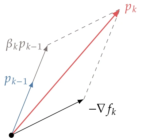
Figure 4.42:The conjugate gradient search direction update combines the steepest-descent direction with the previous conjugate gradient direction.
One option to compute a that achieves conjugacy is given by the Fletcher–Reeves formula,
This formula is derived in Iterative Methods as Equation B.40 in the context of linear solvers. Here, we replace the residual of the linear system with the gradient of the quadratic because they are equivalent.
Using the directions given by Equation 4.56 and the step lengths given by Equation 4.54, we can minimize a quadratic in steps, where is the size of . The minimization shown in Figure 4.41 starts with the steepest-descent direction and then computes one update to converge to the minimum in two iterations using exact line searches. The linear conjugate gradient method is detailed in Algorithm 2.
However, we are interested in minimizing general nonlinear functions. We can adapt the linear conjugate gradient method to the nonlinear case by doing the following:
Use the gradient of the nonlinear function in the search direction update (Equation 4.56) and the expression for (Equation 4.57). This gradient can be computed using any of the methods in Chapter 6.
Perform an inexact line search instead of doing the exact line search. This frees us from providing the Hessian vector products required for an exact line search (see Equation 4.54). A line search that satisfies the strong Wolfe conditions is a good choice, but we need a stricter range in the sufficient decrease and sufficient curvature parameters ().[9] This stricter requirement on is necessary with the Fletcher–Reeves formula (Equation 4.57) to ensure descent directions. As a first guess for in the line search, we can use the same estimate proposed for steepest descent (Equation 4.43).
Reset the search direction periodically back to the steepest-descent direction. In practice, resetting is often helpful to remove old information that is no longer useful. Some methods reset every iterations, motivated by the fact that the linear case only generates conjugate vectors. A more mathematical approach resets the direction when
The full procedure is given in Algorithm 4.6. As with steepest descent, we may use normalized search directions.
The nonlinear conjugate gradient method is no longer guaranteed to converge in steps like its linear counterpart, but it significantly outperforms the steepest-descent method. The change required relative to steepest descent is minimal: save information on the search direction and gradient from the previous iteration, and add the term to the search direction update. Therefore, there is rarely a reason to prefer steepest descent. The parameter can be interpreted as a “damping parameter” that prevents each search direction from varying too much relative to the previous one. When the function steepens, the damping becomes larger, and vice versa.
The formula for in Equation 4.57 is only one of several options. Another well-known option is the Polak–Ribière formula, which is given by
The conjugate gradient method with the Polak–Ribière formula tends to converge more quickly than with the Fletcher–Reeves formula, and this method does not require the more stringent range for . However, regardless of the value of , the strong Wolfe conditions still do not guarantee that is a descent direction ( might become negative). This issue can be addressed by forcing to remain nonnegative:
This equation automatically triggers a reset whenever (see Equation 4.56), so in this approach, other checks on resetting can be removed from Algorithm 4.6.
4.4.3 Newton’s Method
The steepest-descent and conjugate gradient methods use only first-order information (the gradient). Newton’s method uses second-order (curvature) information to get better estimates for search directions. The main advantage of Newton’s method is that, unlike first-order methods, it provides an estimate of the step length because the curvature predicts where the function derivative is zero.
In Section 3.8, we presented Newton’s method for solving nonlinear equations. Newton’s method for minimizing functions is based on the same principle, but instead of solving , we solve for .
As in Section 3.8, we can derive Newton’s method for one-dimensional function minimization from the Taylor series approximation,
We now include a second-order term to get a quadratic that we can minimize. We minimize this quadratic approximation by differentiating with respect to the step and setting the derivative to zero, which yields
Thus, the Newton update is
We could also derive this equation by taking Newton’s method for root finding (Equation 3.24) and replacing with .
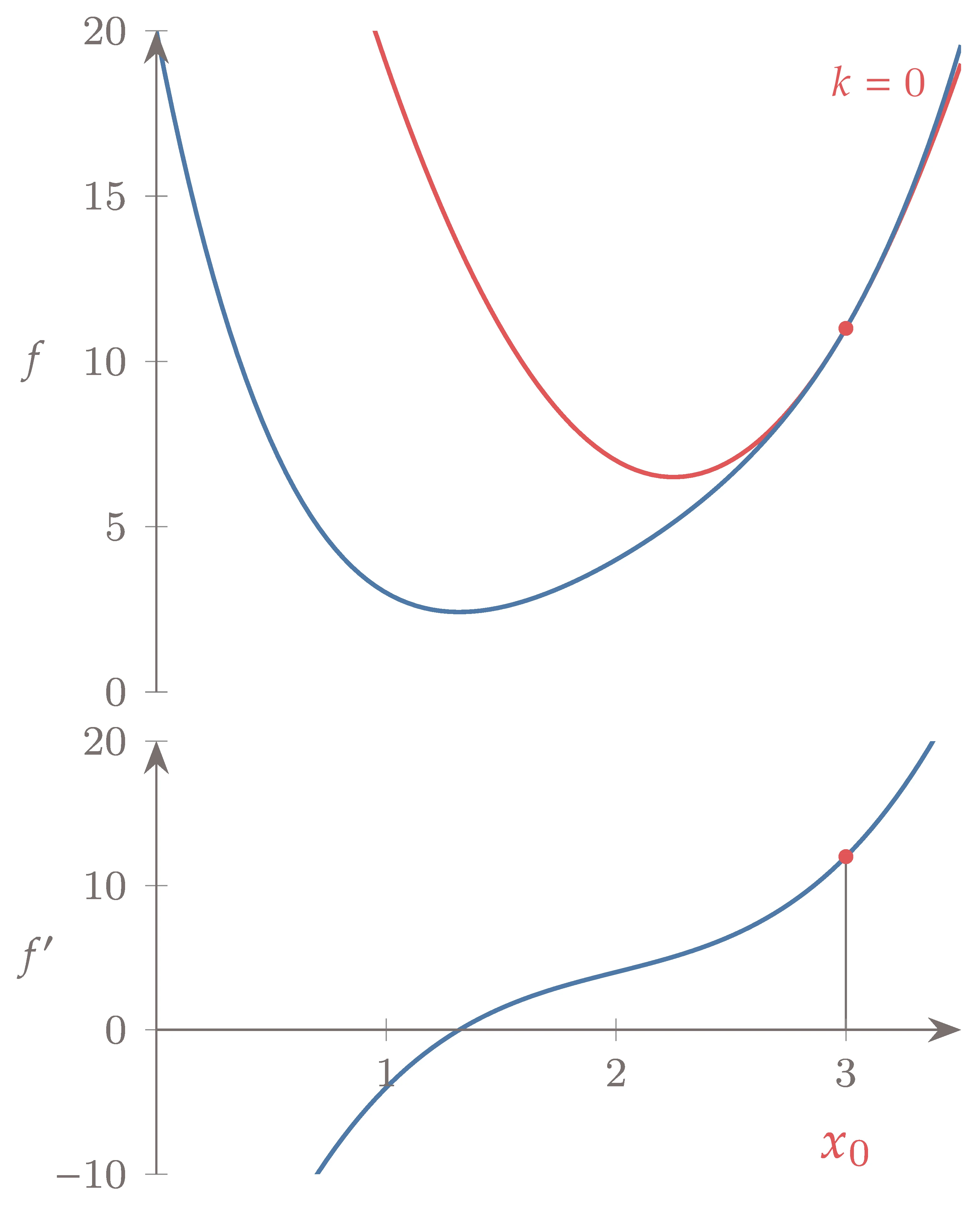
Figure 4.44:Newton’s method for finding roots can be adapted for function minimization by formulating it to find a zero of the derivative. We step to the minimum of a quadratic at each iteration (top) or equivalently find the root of the function’s first derivative (bottom).
Like the one-dimensional case, we can build an -dimensional Taylor series expansion about the current design point:
where is a vector centered at . Similar to the one-dimensional case, we can find the step that minimizes this quadratic model by taking the derivative with respect to and setting that equal to zero:
Thus, each Newton step is the solution of a linear system where the matrix is the Hessian,
This linear system is analogous to the one used for solving nonlinear systems with Newton’s method (Equation 3.30), except that the Jacobian becomes the Hessian, the residual is the gradient, and the design variables replace the states. We can use any of the linear solvers mentioned in Section 3.6 and to solve this system.
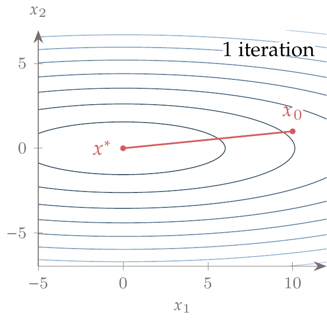
Figure 4.45:Iteration history for a quadratic function using an exact line search and Newton’s method. Unsurprisingly, only one iteration is required.
When minimizing the quadratic function from Example 4.10, Newton’s method converges in one step for any value of , as shown in Figure 4.45. Thus, Newton’s method is scale invariant
Because the function is quadratic, the quadratic “approximation” from the Taylor series is exact, so we can find the minimum in one step. It will take more iterations for a general nonlinear function, but using curvature information generally yields a better search direction than first-order methods. In addition, Newton’s method provides a step length embedded in because the quadratic model estimates the stationary point location. Furthermore, Newton’s method exhibits quadratic convergence.
Although Newton’s method is powerful, it suffers from a few issues in practice. One issue is that the Newton step does not necessarily result in a function decrease. This issue can occur if the Hessian is not positive definite or if the quadratic predictions overshoot because the actual function has more curvature than predicted by the quadratic approximation. Both of these possibilities are illustrated in Figure 4.46.
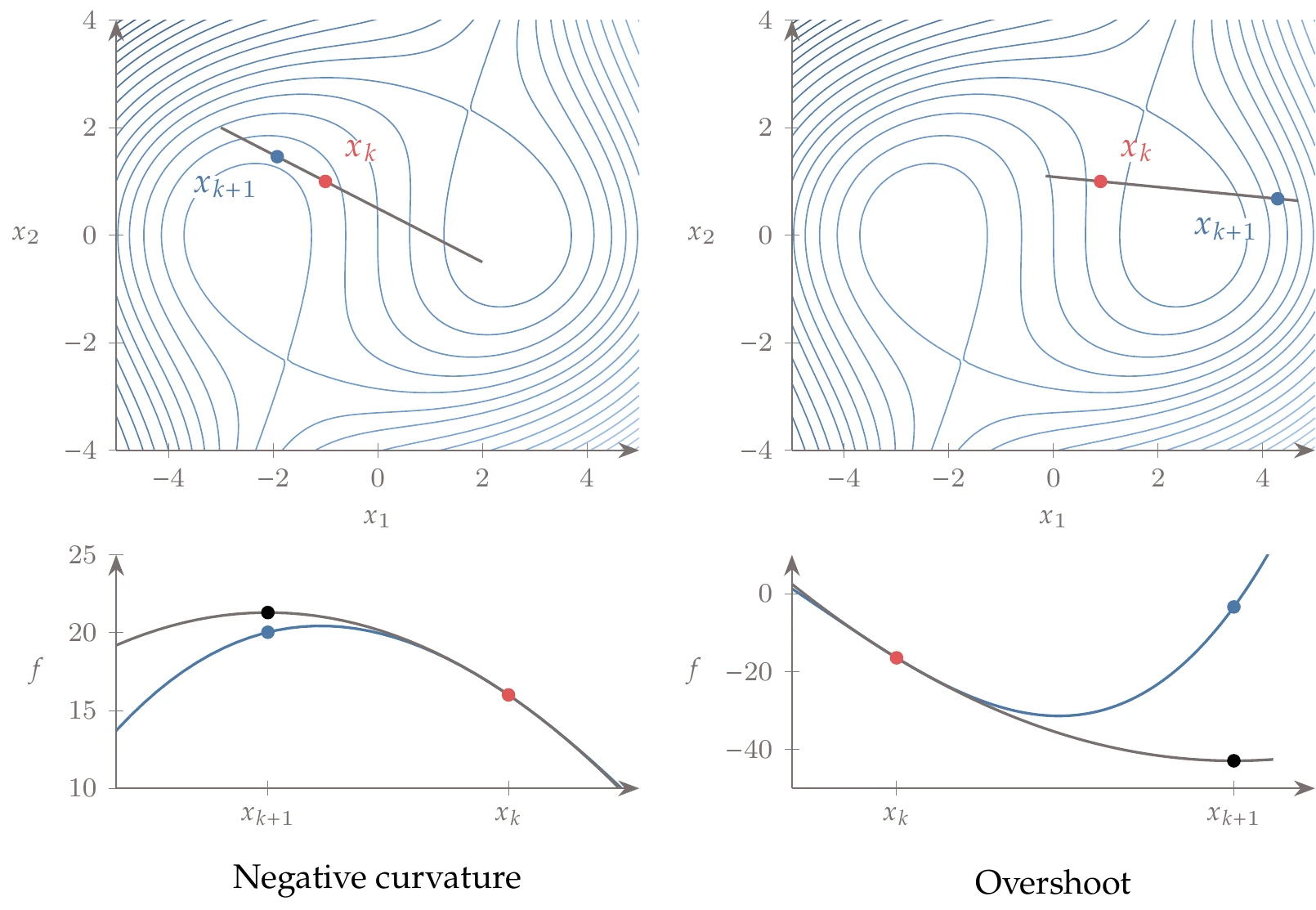
Figure 4.46:Newton’s method in its pure form is vulnerable to negative curvature (in which case it might step away from the minimum) and overshooting (which might result in a function increase).
If the Hessian is not positive definite, the step might not even be in a descent direction. Replacing the real Hessian with a positive-definite Hessian can mitigate this issue. The quasi-Newton methods in the next section force a positive-definite Hessian by construction.
To fix the overshooting issue, we can use a line search instead of blindly accepting the Newton step length. We would set , with as the first guess for the step length. In this case, we have a much better guess for compared with the steepest-descent or conjugate gradient cases because this guess is based on the local curvature. Even if the first step length given by the Newton step overshoots, the line search would find a point with a lower function value.
The trust-region methods in Section 4.5 address both of these issues by minimizing the function approximation within a specified region around the current iteration.
Another major issue with Newton’s method is that the Hessian can be difficult or costly to compute. Even if available, the solution of the linear system in Equation 4.65 can be expensive. Both of these considerations motivate the quasi-Newton methods, which we explain next.
4.4.4 Quasi-Newton Methods
As mentioned in Section 4.4.3, Newton’s method is efficient because the second-order information results in better search directions, but it has the significant shortcoming of requiring the Hessian. Quasi-Newton methods are designed to address this issue. The basic idea is that we can use first-order information (gradients) along each step in the iteration path to build an approximation of the Hessian.
In one dimension, we can adapt the secant method (see Equation 3.26) for function minimization. Instead of estimating the first derivative, we now estimate the second derivative (curvature) using two successive first derivatives, as follows:
Then we can use this approximation in the Newton step (Equation 4.63) to obtain an iterative procedure that requires only first derivatives instead of first and second derivatives.
The quadratic approximation based on this approximation of the second derivative is
Taking the derivative of this approximation with respect to , we get
For , which corresponds to , we get , which tells us that the slope of the approximation matches the slope of the actual function at , as expected.
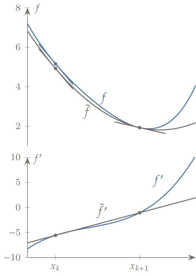
Figure 4.48:The quadratic approximation based on the secant method matches the slopes at the two last points and the function value at the last point.
Also, by stepping backward to by setting , we find that . Thus, the nature of this approximation is such that it matches the slope of the actual function at the last two points, as shown in Figure 4.48.
In dimensions, things are more involved, but the principle is the same: use first-derivative information from the last two points to approximate second-derivative information. Instead of iterating along the -axis as we would in one dimension, the optimization in dimensions follows a sequence of steps (as shown in Figure 4.1) for the separate line searches. We have gradients at the endpoints of each step, so we can take the difference between the gradients at those points to get the curvature along that direction. The question is: How do we update the Hessian, which is expressed in the coordinate system of , based on directional curvatures in directions that are not necessarily aligned with the coordinate system?
Quasi-Newton methods use the quadratic approximation of the objective function,
where is an approximation of the Hessian.
Similar to Newton’s method, we minimize this quadratic with respect to , which yields the linear system
We solve this linear system for , but instead of accepting it as the final step, we perform a line search in the direction. Only after finding a step size that satisfies the strong Wolfe conditions do we update the point using
Quasi-Newton methods update the approximate Hessian at every iteration based on the latest information using an update of the form
where the update is a function of the last two gradients.
The first Hessian approximation is usually set to the identity matrix (or a scaled version of it), which yields a steepest-descent direction for the first line search (set in Equation 4.71 to verify this).
We now develop the requirements for the approximate Hessian update. Suppose we just obtained the new point after a line search starting from in the direction . We can write the new quadratic based on an updated Hessian as follows:
We can assume that the new point’s function value and gradient are given, but we do not have the new approximate Hessian yet. Taking the gradient of this quadratic with respect to , we obtain
In the single-variable case, we observed that the quadratic approximation based on the secant method matched the slope of the actual function at the last two points. Therefore, it is logical to require the -dimensional quadratic based on the approximate Hessian to match the gradient of the actual function at the last two points.
The gradient of the new approximation (Equation 4.75) matches the gradient at the new point by construction (just set ). To find the gradient predicted by the new approximation (Equation 4.75) at the previous point , we set (which is a backward step from the end of the last line search to the start of the line search) to get
Now, we enforce that this must be equal to the actual gradient at that point,
To simplify the notation, we define the step as
and the difference in the gradient as
Figure 4.49 shows the step and the corresponding gradients.
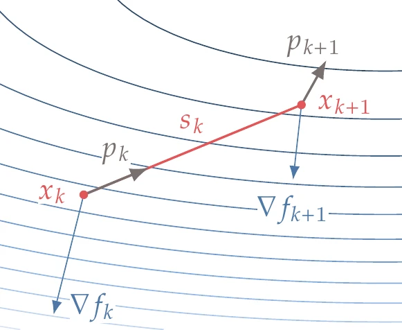
Figure 4.49:Quasi-Newton methods use the gradient at the endpoint of each step to estimate the curvature in the step direction and update an approximation of the Hessian.
Rewriting Equation 4.77 using this notation, we get
This is called the secant equation and is a fundamental requirement for quasi-Newton methods. The result is intuitive when we recall the meaning of the product of the Hessian with a vector (Equation 4.12): it is the rate of change of the Hessian in the direction defined by that vector. Thus, it makes sense that the rate of change of the curvature predicted by the approximate Hessian should match the difference between the gradients.[10]
We need to be positive definite. Using the secant equation (Equation 4.80) and the definition of positive definiteness (), we see that this requirement implies that the predicted curvature is positive along the step; that is,
This is called the curvature condition, and it is automatically satisfied if the line search finds a step that satisfies the strong Wolfe conditions.
The secant equation (Equation 4.80) is a linear system of equations where the step and the gradients are known. However, there are unknowns in the approximate Hessian matrix (recall that it is symmetric), so this equation is not sufficient to determine the elements of . The requirement of positive definiteness adds one more equation, but those are not enough to determine all the unknowns, leaving us with an infinite number of possibilities for .
To find a unique , we rationalize that among all the matrices that satisfy the secant equation (Equation 4.80), should be the one closest to the previous approximate Hessian, . This makes sense intuitively because the curvature information gathered in one step is limited (because it is along a single direction) and should not change the Hessian approximation more than necessary to satisfy the requirements.
The original quasi-Newton update, known as DFP, was first proposed by Davidon and then refined by Fletcher and also Powell (see historical note in Section 2.3).56 The DFP update formula has been superseded by the BFGS formula, which was independently developed by Broyden, Fletcher, Goldfarb, and Shanno.78910 BFGS is currently considered the most effective quasi-Newton update, so we focus on this update. However, Section C.2.1 has more details on DFP.
The formal derivation of the BFGS update formula is rather involved, so we do not include it here. Instead, we work through an informal derivation that provides intuition about this update and quasi-Newton methods in general. We also include more details in Section C.2.2.
Recall that quasi-Newton methods add an update to the previous Hessian approximation (Equation 4.73). One way to think about an update that yields a matrix close to the previous one is to consider the rank of the update, . The lower the rank of the update, the closer the updated matrix is to the previous one. Also, the curvature information contained in this update is minimal because we are only gathering information in one direction for each update. Therefore, we can reason that the rank of the update matrix should be the lowest possible rank that satisfies the secant equation (Equation 4.80).
The update must be symmetric and positive definite to ensure a symmetric positive-definite Hessian approximation. If we start with a symmetric positive-definite approximation, then all subsequent approximations remain symmetric and positive definite. As it turns out, it is possible to derive a rank 1 update matrix that satisfies the secant equation, but this update is not guaranteed to be positive definite. However, we can get positive definiteness with a rank 2 update.
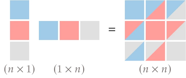
Figure 4.50:The self outer product of a vector produces a symmetric matrix of rank 1.
We can obtain a symmetric rank 2 update by adding two symmetric rank 1 matrices. One convenient way to obtain a symmetric rank 1 matrix is to perform a self outer product of a vector, which takes a vector of size and multiplies it with its transpose to obtain an matrix, as shown in Figure 4.50. Matrices resulting from vector outer products have rank 1 because all the columns are linearly dependent.
With two linearly independent vectors ( and ), we can get a rank 2 update using
where and are scalar coefficients. Substituting this into the secant equation (Equation 4.80), we have
Because the new information about the function is encapsulated in the vectors and , we can reason that and should be based on these vectors. It turns out that using on its own does not yield a useful update (one term cancels out), but does. Setting and in Equation 4.83 yields
Rearranging this equation, we have
Because the vectors and are not parallel in general (because the secant equation applies to , not to ), the only way to guarantee this equality is to set the terms in parentheses to zero. Thus, the scalar coefficients are
Substituting these coefficients and the chosen vectors back into Equation 4.82, we get the BFGS update,
Although we did not explicitly enforce positive definiteness, the rank 2 update is positive definite, and therefore, all the Hessian approximations are positive definite, as long as we start with a positive-definite approximation.
Now recall that we want to solve the linear system that involves this matrix (Equation 4.71), so it would be more efficient to approximate the inverse of the Hessian directly instead. The inverse can be found analytically from the update (Equation 4.87) using the Sherman–Morrison–Woodbury formula.[11]Defining as the approximation of the inverse of the Hessian, the final result is
where
Figure 4.51 shows the sizes of the vectors and matrices involved in this equation.
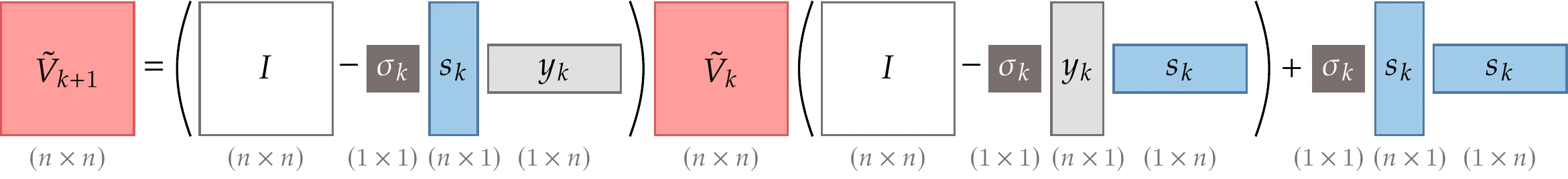
Figure 4.51:Sizes of each term of the BFGS update (Equation 4.88).
Now we can replace the potentially costly solution of the linear system (Equation 4.71) with the much cheaper matrix-vector product,
where is the estimate for the inverse of the Hessian.
Algorithm 4.7 details the steps for the BFGS algorithm. Unlike first-order methods, we should not normalize the direction vector because the length of the vector is meaningful. Once we have curvature information, the quasi-Newton step should give a reasonable estimate of where the function slope flattens. Thus, as advised for Newton’s method, we set . Alternatively, this would be equivalent to using a normalized direction vector and then setting to the initial magnitude of . However, optimization algorithms in practice use to signify that a full (quasi-) Newton step was accepted (see Tip 4.5).
As discussed previously, we need to start with a positive-definite estimate to maintain a positive-definite inverse Hessian. Typically, this is the identity matrix or a weighted identity matrix, for example:
This makes the first step a normalized steepest-descent direction:
In a practical algorithm, might require occasional resets to the scaled identity matrix. This is because as we iterate in the design space, curvature information gathered far from the current point might become irrelevant and even counterproductive. The trigger for this reset could occur when the directional derivative is greater than some threshold. That would mean that the slope along the search direction is shallow; in other words, the search direction is close to orthogonal to the steepest-descent direction.
Another well-known quasi-Newton update is the symmetric rank 1 (SR1) update, which we derive in Section C.2.3. Because the update is rank 1, it does not guarantee positive definiteness. Why would we be interested in a Hessian approximation that is potentially indefinite? In practice, the matrices produced by SR1 have been found to approximate the true Hessian matrix well, often better than BFGS. This alternative is more common in trust-region methods (see Section 4.5), which depend more strongly on an accurate Hessian and do not require positive definiteness. It is also sometimes used for constrained optimization problems where the Hessian of the Lagrangian is often indefinite, even at the minimizer.
4.4.5 Limited-Memory Quasi-Newton Methods
When the number of design variables is large (millions or billions), it might not be possible to store the Hessian inverse approximation matrix in memory. This motivates limited-memory quasi-Newton methods, which make it possible to handle such problems. In addition, these methods also improve the computational efficiency of medium-sized problems (hundreds or thousands of design variables) with minimal sacrifice in accuracy.
Recall that we are only interested in the matrix-vector product to find each search direction using Equation 4.90. As we will see in this section, we can compute this product without ever actually forming the matrix . We focus on doing this for the BFGS update because this is the most popular approach (known as L-BFGS), although similar techniques apply to other quasi-Newton update formulas.
The BFGS update (Equation 4.88) is a recursive sequence:
where
If we save the sequence of and vectors and specify a starting value for , we can compute any subsequent . Of course, what we want is , which we can also compute using an algorithm with the recurrence relationship. However, such an algorithm would not be advantageous from the memory-usage perspective because we would have to store a long sequence of vectors and a starting matrix.
To reduce the memory usage, we do not store the entire history of vectors. Instead, we limit the storage to the last vectors for and . In practice, is usually between 5 and 20.
Next, we make the starting Hessian diagonal such that we only require vector storage (or scalar storage if we make all entries in the diagonal equal). A common choice is to use a scaled identity matrix, which just requires storing one number,
where the and correspond to the previous iteration. Algorithm 4.8 details the procedure.
Using this technique, we no longer need to bear the memory cost of storing a large matrix or incur the computational cost of a large matrix-vector product. Instead, we store a small number of vectors and require fewer vector-vector products (a cost that scales linearly with rather than quadratically).
The number of major iterations is not always an effective way to compare performance. For example, Newton’s method takes fewer major iterations, but each iteration in Newton’s method is more expensive than each iteration in the quasi-Newton method. This is because Newton’s method requires a linear solution, which is an operation, as opposed to a matrix-vector multiplication, which is an operation. For a small problem like the two-dimensional Rosenbrock function, this is an insignificant difference, but this is a significant difference in computational effort for large problems. Additionally, each major iteration includes a line search, and depending on the quality of the search direction, the number of function calls contained in each iteration will differ.
Poor scaling causes premature convergence for various reasons. In Example 4.19, it was because convergence was based on a tolerance relative to the starting gradient, and some gradient components were much smaller than others. When using an absolute tolerance, premature convergence can occur when the gradients are small to begin with (because of the scale of the problem, not because they are near an optimum). When the scaling is poor, the optimizer is even more dependent on accurate gradients to navigate the narrow regions of function improvement.
Larger engineering simulations are usually more susceptible to numerical noise due to iteration loops, solver convergence tolerances, and longer computational procedures. Another issue arises when the derivatives are not computed accurately. In these cases, poorly scaled problems struggle because the line search directions are not accurate enough to yield a decrease, except for tiny step sizes.
Most practical optimization algorithms terminate early when this occurs, not because the optimality conditions are satisfied but because the step sizes or function changes are too small, and progress is stalled (see Tip 4.1). A lack of attention to scaling is one of the most frequent causes of poor solutions in engineering optimization problems.
4.5 Trust-Region Methods
In Section 4.2, we mentioned two main approaches for unconstrained gradient-based optimization: line search and trust region. We described the line search in Section 4.3 and the associated methods for computing search directions in Section 4.4. Now we describe trust-region methods, also known as restricted-step methods. The main motivation for trust-region methods is to address the issues with Newton’s method (see Section 4.4.3) and quasi-Newton updates that do not guarantee a positive definite-Hessian approximation (e.g., SR1, which we briefly described in Section 4.4.4).
The trust-region approach is fundamentally different from the line search approach because it finds the direction and distance of the step simultaneously instead of finding the direction first and then the distance. The trust-region approach builds a model of the function to be minimized and then minimizes the model within a trust region, within which we trust the model to be good enough for our purposes.
The most common model is a local quadratic function, but other models may be used. When using a quadratic model based on the function value, gradient, and Hessian at the current iteration, the method is similar to Newton’s method.
Figure 4.60:Trust-region methods minimize a model within a trust region for each iteration, and then they update the trust-region size and the model before the next iteration.
The trust region is centered about the current iteration point and can be defined as an -dimensional box, sphere, or ellipsoid of a given size. Each trust-region iteration consists of the following main steps:
Create or update the model about the current point.
Minimize the model within the trust region.
Move to the new point, update values, and adapt the size of the trust region.
These steps are illustrated in Figure 4.60, and they are repeated until convergence. Figure 4.61 shows the steps to minimize the bean function, where the circles show the trust regions for each iteration.
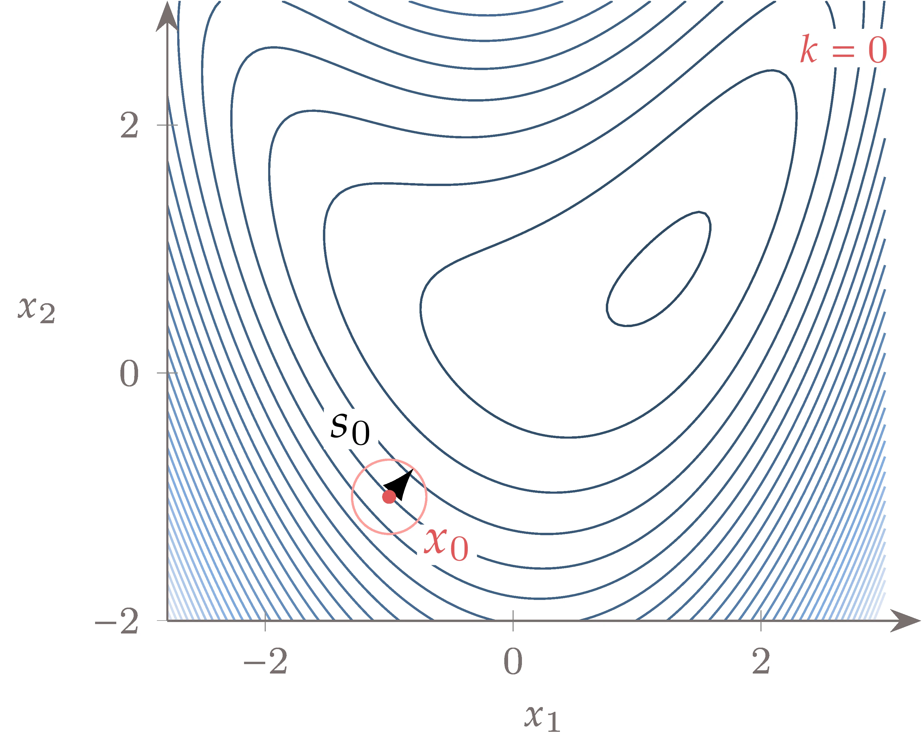
Figure 4.61:Path for the trust-region approach showing the circular trust regions at each step.
The trust-region subproblem solved at each iteration is
where is the local trust-region model, is the step from the current iteration point, and is the size of the trust region. We use instead of to indicate that this is a step vector and not simply the direction vector used in methods based on a line search.
The subproblem (Equation 4.97) defines the trust region as a norm. The Euclidean norm, , defines a spherical trust region and is the most common type of trust region. Sometimes -norms are used instead because they are easy to apply, but 1-norms are rarely used because they are just as complex as 2-norms but introduce sharp corners that can be problematic.11 The shape of the trust region is dictated by the norm (see Figure A.8) and can significantly affect the convergence rate. The ideal trust-region shape depends on the local function space, and some algorithms allow for the trust-region shape to change throughout the optimization.
4.5.1 Quadratic Model with Spherical Trust Region
Using a quadratic trust-region model and the Euclidean norm, we can define the more specific subproblem:
where is the approximate (or true) Hessian at our current iterate. This problem has a quadratic objective and quadratic constraints and is called a quadratically constrained quadratic program (QCQP).
If the problem is unconstrained and is positive definite, we can get to the solution using a single step, . However, because of the constraints, there is no analytic solution for the QCQP. Although the problem is still straightforward to solve numerically (because it is a convex problem; see Section 11.4), it requires an iterative solution approach with multiple factorizations.
Similar to the line search, where we only obtain a sufficiently good point instead of finding the exact minimum, in the trust-region subproblem, we seek an approximate solution to the QCQP. Including the trust-region constraint allows us to omit the requirement that be positive definite, which is used in most quasi-Newton methods. We do not detail approximate solution methods to the QCQP, but there are various options.11124
Figure 4.62 compares the bean function with a local quadratic model, which is built using information about the point where the arrow originates. The trust-region step seeks the minimum of the local quadratic model within the circular trust region. Unlike line search methods, as the size of the trust region changes, the direction of the step (the solution to Equation 4.98) might also change, as shown on the right panel of Figure 4.62.
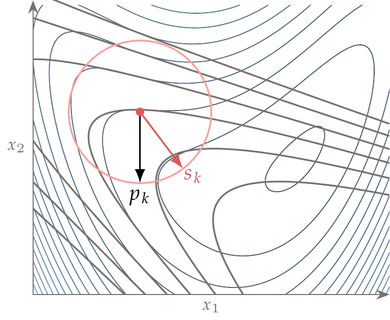
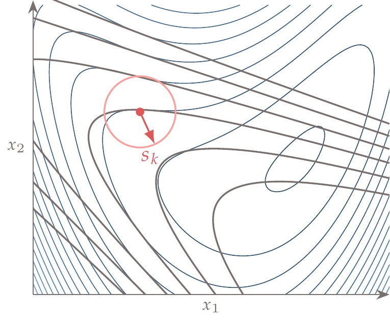
Figure 4.62:Quadratic model (gray contours) compared to the actual function (blue contours), and two different different trust region sizes (red circles). The trust-region step finds the minimum of the quadratic model while remaining within the trust region. The steepest-descent direction is shown for comparison.
4.5.2 Trust-Region Sizing Strategy
This section presents an algorithm for updating the size of the trust region at each iteration. The trust region can grow, shrink, or remain the same, depending on how well the model predicts the actual function decrease. The metric we use to assess the model is the actual function decrease divided by the expected decrease:
The denominator in this definition is the expected decrease, which is always positive. The numerator is the actual change in the function, which could be a reduction or an increase. An value close to unity means that the model agrees well with the actual function. An value larger than 1 is fortuitous and means that the actual decrease was even greater than expected. A negative value of means that the function actually increased at the expected minimum, and therefore the model is not suitable.
The trust-region sizing strategy in Algorithm 4.9 determines the size of the trust region at each major iteration based on the value of . The parameters in this algorithm are not derived from any theory; instead, they are empirical. This example uses the basic procedure from Nocedal & Wright (2006) with the parameters recommended by Conn et al. (2000)
The initial value of is usually 1, assuming the problem is already well scaled. One way to rationalize the trust-region method is that the quadratic approximation of a nonlinear function is guaranteed to be reasonable only within a limited region around the current point . Thus, we minimize the quadratic function within a region around within which we trust the quadratic model.
When our model performs well, we expand the trust region. When it performs poorly, we shrink the trust region. If we shrink the trust region sufficiently, our local model will eventually be a good approximation of the actual function, as dictated by the Taylor series expansion.
We should also set a maximum trust-region size () to prevent the trust region from expanding too much. Otherwise, it may take too long to reduce the trust region to an acceptable size over other portions of the design space where a smaller trust region is needed.
The same convergence criteria used in other gradient-based methods are applicable.[14]
4.5.3 Comparison with Line Search Methods
Trust-region methods are typically more strongly dependent on accurate Hessians than are line search methods. For this reason, they are usually only effective when exact gradients (or better yet, an exact Hessian) can be supplied. Many optimization packages require the user to provide the full Hessian, or at least the gradients, to use a trust-region approach. Trust-region methods usually require fewer iterations than quasi-Newton methods with a line search, but each iteration is more computationally expensive because they require at least one matrix factorization.
Scaling can also be more challenging with trust-region approaches. Newton’s method is invariant with scaling, but a Euclidean trust-region constraint implicitly assumes that the function changes in each direction at a similar rate. Some enhancements try to address this issue through elliptical trust regions rather than spherical ones.
4.6 Summary
Gradient-based optimization is powerful because gradients make it possible to efficiently navigate -dimensional space in a series of steps converging to an optimum. The gradient also determines when the optimum has been reached, which is when the gradient is zero.
Gradients provide only local information, so an approach that ensures a function decrease when stepping away from the current point is required. There are two approaches to ensure this: line search and trust region. Algorithms based on a line search have two stages: finding an appropriate search direction and determining how far to step in that direction. Trust-region algorithms minimize a surrogate function within a finite region around the current point. The region expands or contracts, depending on how well the optimization within the previous iteration went. Gradient-based optimization algorithms based on a line search are more prevalent than trust-region methods, but trust-region methods can be effective when second derivatives are available.
There are different options for determining the search direction for each line search using gradient information. Although the negative gradient points in the steepest-descent direction, following this direction is not the best approach because it is prone to oscillations. The conjugate gradient method dampens these oscillations and thus converges much faster than steepest descent.
Second-order methods use curvature information, which dramatically improves the rate of convergence. Newton’s method converges quadratically but requires the Hessian of the function, which can be prohibitive. Quasi-Newton methods circumvent this requirement by building an approximation of the inverse of the Hessian based on changes in the gradients along the optimization path. Quasi-Newton methods also avoid matrix factorization, requiring matrix-vector multiplication instead. Because they are much less costly while achieving better than linear convergence, quasi-Newton methods are widely used. Limited-memory quasi-Newton methods can be used when the problem is too large to fit in computer memory.
The line search in a given direction does not seek to find a minimum because this is not usually worthwhile. Instead, it seeks to find a “good enough” point that sufficiently decreases the function and the slope. Once such a point is found, we select a new search direction and repeat the process. Second-order methods provide a guess for the first step length in the line search that further improves overall convergence.
This chapter provides the building blocks for the gradient-based constrained optimization covered in the next chapter.
Problems
In this book, most of the illustrations and examples are based on two-dimensional problems because they are easy to visualize. However, the principles and methods apply to dimensions.
The discovery and proof of the symmetry of second derivatives property has a long history.1
For a more extensive introduction to the Taylor series, see Taylor Series Expansion.
For other approaches to determine if a matrix is positive definite, see Section A.6.
This algorithm, and others in this section, use a basic convergence check for simplicity. See the end of Section 4.1.4 for better alternatives and additional exit criteria.
If can be negative, a transformation is required to ensure that the logarithm argument is always positive.
The secant equation is also known as the quasi-Newton condition.
This formula is also known as the Woodbury matrix identity. Given a matrix and an update to that matrix, it yields an explicit expression for the inverse of the updated matrix in terms of the inverses of the matrix and the update (see Section C.3).
Section D.1.8 has details on this problem.
The “bean” function we used in previous examples is a milder version of the Rosenbrock function.
11 provide more detail on trust-region problems, including trust-region norms and scaling, approaches to solving the trust-region subproblem, extensions to the model, and other important practical considerations.
Another option to smooth the max of multiple functions is aggregation, which is detailed in Section 5.7.
This problem was mentioned in Section 2.2 as one of the problems that inspired developments in calculus of variations.
- Higgins, T. J. (1940). A note on the history of mixed partial derivatives. Scripta Mathematica, 7, 59–62.
- Hager, W. W., & Zhang, H. (2005). A new conjugate gradient method with guaranteed descent and an efficient line search. SIAM Journal on Optimization, 16(1), 170–192. 10.1137/030601880
- Moré, J. J., & Thuente, D. J. (1994). Line search algorithms with guaranteed sufficient decrease. ACM Transactions on Mathematical Software (TOMS), 20(3), 286–307. 10.1145/192115.192132
- Nocedal, J., & Wright, S. J. (2006). Numerical Optimization (2nd ed.). Springer. 10.1007/978-0-387-40065-5
- Davidon, W. C. (1991). Variable metric method for minimization. SIAM Journal on Optimization, 1(1), 1–17. 10.1137/0801001
- Fletcher, R., & Powell, M. J. D. (1963). A rapidly convergent descent method for minimization. The Computer Journal, 6(2), 163–168. 10.1093/comjnl/6.2.163
- Broyden, C. G. (1970). The convergence of a class of double-rank minimization algorithms 1. General considerations. IMA Journal of Applied Mathematics, 6(1), 76–90. 10.1093/imamat/6.1.76
- Fletcher, R. (1970). A new approach to variable metric algorithms. The Computer Journal, 13(3), 317–322. 10.1093/comjnl/13.3.317
- Goldfarb, D. (1970). A family of variable-metric methods derived by variational means. Mathematics of Computation, 24(109), 23–23. 10.1090/s0025-5718-1970-0258249-6
- Shanno, D. F. (1970). Conditioning of quasi-Newton methods for function minimization. Mathematics of Computation, 24(111), 647–647. 10.1090/s0025-5718-1970-0274029-x
- Conn, A. R., Gould, N. I. M., & Toint, Ph. L. (2000). Trust Region Methods. SIAM.
- Steihaug, T. (1983). The conjugate gradient method and trust regions in large scale optimization. SIAM Journal on Numerical Analysis, 20(3), 626–637. 10.1137/0720042