Appendix: Mathematics Background
This appendix briefly reviews various mathematical concepts used throughout the book.
A.1 Taylor Series Expansion
Series expansions are representations of a given function in terms of a series of other (usually simpler) functions. One common series expansion is the Taylor series, which is expressed as a polynomial whose coefficients are based on the derivatives of the original function at a fixed point.
The Taylor series is a general tool that can be applied whenever the function has derivatives. We can use this series to estimate the value of the function near the given point, which is useful when the function is difficult to evaluate directly. The Taylor series is used to derive algorithms for finding the zeros of functions and algorithms for minimizing functions in Chapter 4 and Chapter 5.
To derive the Taylor series, we start with an infinite polynomial series about an arbitrary point, , to approximate the value of a function at using
We can make this approximation exact at by setting the first coefficient to . To find the appropriate value for , we take the first derivative to get
which means that we need to obtain an exact derivative at . To derive the other coefficients, we systematically take the derivative of both sides and the appropriate value of the first nonzero term (which is always constant). Identifying the pattern yields the general formula for the th-order coefficient:
Substituting this into the polynomial in Equation A.1 yields the Taylor series
The series is typically truncated to use terms up to order ,
which yields an approximation with a truncation error of order . In optimization, it is common to use the first three terms (up to ) to get a quadratic approximation.
The Taylor series in multiple dimensions is similar to the single-variable case but more complicated. The first derivative of the function becomes a gradient vector, and the second derivatives become a Hessian matrix. Also, we need to define a direction along which we want to approximate the function because that information is not inherent like it is in a one-dimensional function. The Taylor series expansion in dimensions along a direction can be written as
where is a scalar that determines how far to go in the direction .
In matrix form, we can write
where is the Hessian matrix.
A.2 Chain Rule, Total Derivatives, and Differentials
The single-variable chain rule is needed for differentiating composite functions. Given a composite function, , the derivative with respect to the variable is
If a function depends on more than one variable, then we need to distinguish between partial and total derivatives. For example, if , then is a function of two variables: and . The application of the chain rule for this function is
where indicates a partial derivative, and is a total derivative. When taking a partial derivative, we take the derivative with respect to only that variable, treating all other variables as constants. More generally,
The differential of a function represents the linear change in that function with respect to changes in the independent variable. We introduce them here because they are helpful for finding total derivatives of multivariable equations that are implicit.
If function is differentiable, the differential is
where is a nonzero real number (considered small) and is an approximation of the change (due to the linear term in the Taylor series). We can solve for to get . This states that the derivative of with respect to is the differential of divided by the differential of . Strictly speaking, here is not the derivative, although it is written in the same way. The derivative is a symbol, not a fraction. However, for our purposes, we will use these representations interchangeably and treat differentials algebraically. We also write the differentials of functions as
In Example 5, there is no clear advantage in using differentials. However, differentials are more straightforward for finding total derivatives of multivariable implicit equations because there is no need to identify the independent variables. Given an equation, we just need to (1) find the differential of the equation and (2) solve for the derivative of interest. When we want quantities to remain constant, we can set the corresponding differential to zero. Differentials can be applied to vectors (say a vector of size ), yielding a vector of differentials with the same size ( of size ). We use this technique to derive the unified derivatives equation (UDE) in Section 6.9.
A.3 Matrix Multiplication
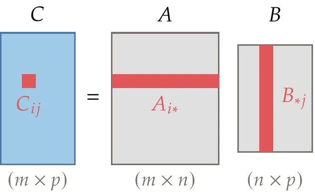
Figure A.3:Matrix product and resulting size.
Consider a matrix of size [1]and a matrix of size . The two matrices can be multiplied together as follows:
where is an matrix. This multiplication is illustrated in Figure A.3. Two matrices can be multiplied only if their inner dimensions are equal ( in this case). The remaining products discussed in this section are just special cases of matrix multiplication, but they are common enough that we discuss them separately.
A.3.1 Vector-Vector Products
In this book, a vector is a column vector; thus, the row vector is represented as . The product of two vectors can be performed in two ways. The more common is called an inner product (also known as a dot product or scalar product). The inner product is a functional, meaning that it is an operator that acts on vectors and produces a scalar. This product is illustrated in Figure A.4. In the real vector space of dimensions, the inner product of two vectors, and , whose dimensions are equal, is defined algebraically as
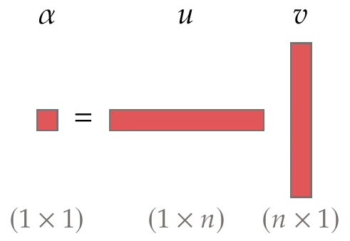
Figure A.4:Dot (or inner) product of two vectors.
The order of multiplication is irrelevant, and therefore,
In Euclidean space, where vectors have magnitude and direction, the inner product is defined as
where represents the 2-norm (Equation A.25), and is the angle between the two vectors.
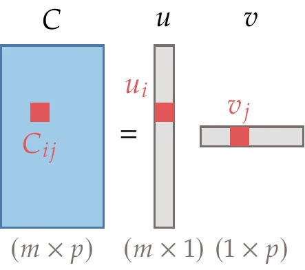
Figure A.5:Outer product of two vectors.
The outer product takes the two vectors and multiplies them element-wise to produce a matrix, as illustrated in Figure A.5. Unlike the inner product, the outer product does not require the vectors to be of the same length. The matrix form is as follows:
The index form is as follows:
Outer products generate rank 1 matrices. They are used in quasi-Newton methods (Section 4.4.4 and ).
A.3.2 Matrix-Vector Products
Consider multiplying a matrix of size by vector of size . The result is a vector of size :
This multiplication is illustrated in Figure A.6.
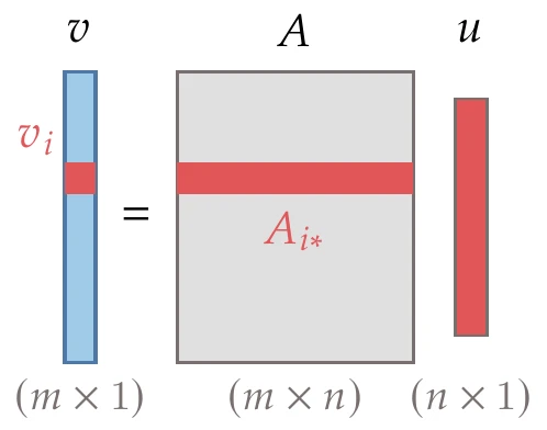
Figure A.6:Matrix-vector product.
The entries in are dot products between the rows of and :
where is the th row of the matrix . Thus, a matrix-vector product transforms a vector in -dimensional space () to a vector in -dimensional space ().
A matrix-vector product can be thought of as a linear combination of the columns of , where the values are the weights:
and are the columns of .
We can also multiply by a vector on the left, instead of on the right:
In this case, a row vector is multiplied with a matrix, producing a row vector.
A.3.3 Quadratic Form (Vector-Matrix-Vector Product)
Another common product is a quadratic form. A quadratic form consists of a row vector, times a matrix, times a column vector, producing a scalar:
The index form is as follows:
In general, a vector-matrix-vector product can have a nonsquare matrix, and the vectors would be two different sizes, but for a quadratic form, the two vectors are identical, and thus is square. Also, in a quadratic form, we assume that is symmetric (even if it is not, only the symmetric part of contributes, so effectively, it acts like a symmetric matrix).
A.4 Four Fundamental Subspaces in Linear Algebra
This section reviews how the dimensions of a matrix in a linear system relate to dimensional spaces.[2] These concepts are especially helpful for understanding constrained optimization (Chapter 5) and build on the review in Section 5.2n-Dimensional Space.
A vector space is the set of all points that can be obtained by linear combinations of a given set of vectors. The vectors are said to span the vector space. A basis is a set of linearly independent vectors that generates all points in a vector space. A subspace is a space of lower dimension than the space that contains it (e.g., a line is a subspace of a plane).
Two vectors are orthogonal if the angle between them is 90 degrees. Then, their dot product is zero. A subspace is orthogonal to another subspace if every vector in is orthogonal to every vector in .
Consider an matrix . The rank () of a matrix is the maximum number of linearly independent row vectors of or, equivalently, the maximum number of linearly independent column vectors. The rank can also be defined as the dimensionality of the vector space spanned by the rows or columns of . For an matrix, .
Through a matrix-vector multiplication , this matrix maps an -vector into an -vector .
Figure A.7 shows this mapping and illustrates the four fundamental subspaces that we now explain.
The column space of a matrix is the vector space spanned by the vectors in the columns of . The dimensionality of this space is given by , where , so the column space is a subspace of -dimensional space. The row space of a matrix is the vector space spanned by the vectors in the rows of (or equivalently, it is the column space of ). The dimensionality of this space is given by , where , so the row space is a subspace of -dimensional space.
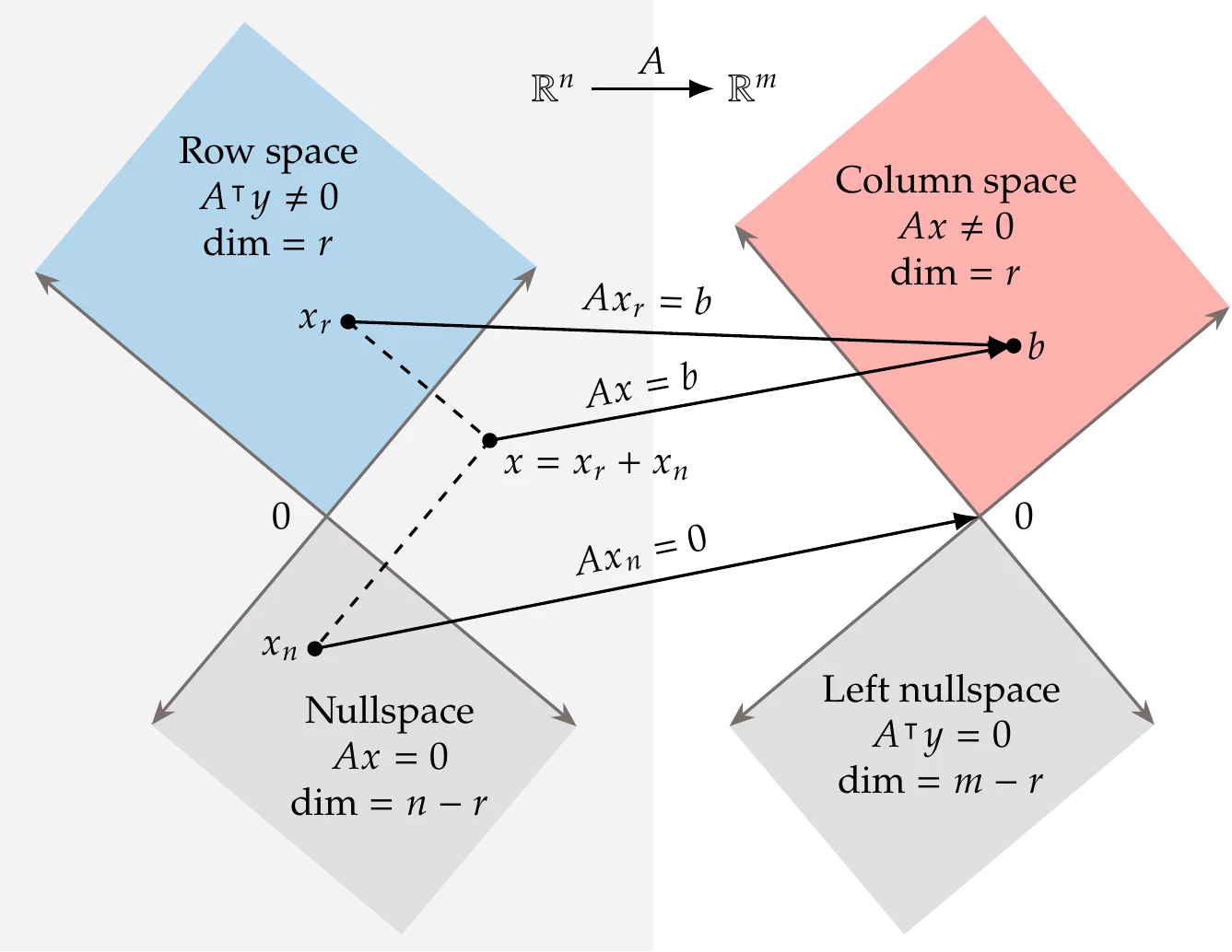
Figure A.7:The four fundamental subspaces of linear algebra. An matrix maps vectors from -space to -space. When the vector is in the row space of the matrix, it maps to the column space of (). When the vector is in the nullspace of , it maps to zero (). Combining the row space and nullspace of , we can obtain any vector in -dimensional space (), which maps to the column space of ().
The nullspace of a matrix is the vector space consisting of all the vectors that are orthogonal to the rows of . Equivalently, the nullspace of is the vector space of all vectors such that . Therefore, the nullspace is orthogonal to the row space of . The dimension of the nullspace of is .
Combining the nullspace and row space of adds up to the whole -dimensional space, that is, , where is in the row space of and is in the nullspace of .
The left nullspace of a matrix is the vector space of all such that . Therefore, the left nullspace is orthogonal to the column space of . The dimension of the left nullspace of is . Combining the left nullspace and column space of adds up to the whole -dimensional space.
A.5 Vector and Matrix Norms
Norms give an idea of the magnitude of the entries in vectors and matrices. They are a generalization of the absolute value for real numbers. A norm is a real-valued function with the following properties:
for all .
if an only if .
for all real numbers .
for all and .
Most common matrix norms also have the property that , although this is not required in general.
We start by defining vector norms, where the vector is . The most familiar norm for vectors is the 2-norm, also known as the Euclidean norm, which corresponds to the Euclidean length of the vector:
Because this norm is used so often, we often omit the subscript and just write . In this book, we sometimes use the square of the 2-norm, which can be written as the dot product,
More generally, we can refer to a class of norms called -norms:
where . Of all the -norms, three are most commonly used: the 2-norm (Equation A.25), the 1-norm, and the -norm. From the previous definition, we see that the 1-norm is the sum of the absolute values of all the entries in :
The application of in the -norm definition is perhaps less obvious, but as , the largest term in that sum dominates all of the others. Raising that quantity to the power of causes the exponents to cancel, leaving only the largest-magnitude component of . Thus, the infinity norm is
The infinity norm is commonly used in optimization convergence criteria.

Figure A.8:Norms for two-dimensional case.
The vector norms are visualized in Figure A.8 for . If , then
It is also possible to assign different weights to each vector component to form a weighted norm:
Several norms for matrices exist. There are matrix norms similar to the vector norms that we defined previously. Namely,
where is the largest eigenvalue of . When is a square symmetric matrix, then
Another matrix norm that is useful but not related to any vector norm is the Frobenius norm, which is defined as the square root of the absolute squares of its elements, that is,
The Frobenius norm can be weighted by a matrix as follows:
This norm is used in the formal derivation of the Broyden–Fletcher–Goldfarb–Shanno (BFGS) update formula (see ).
A.6 Matrix Types
There are several common types of matrices that appear regularly throughout this book. We review some terminology here.
A diagonal matrix is a matrix where all off-diagonal terms are zero. In other words, is diagonal if:
The identity matrix is a special diagonal matrix where all diagonal components are 1.
The transpose of a matrix is defined as follows:
Note that
A symmetric matrix is one where the matrix is equal to its transpose:
The inverse of a matrix, , satisfies
Not all matrices are invertible. Some common properties for inverses are as follows:
A symmetric matrix is positive definite if and only if
for all nonzero vectors . One property of positive-definite matrices is that their inverse is also positive definite.
The positive-definite condition (Equation A.42) can be challenging to verify. Still, we can use equivalent definitions that are more practical.
For example, by choosing appropriate s, we can derive the necessary conditions for positive definiteness:
These are necessary but not sufficient conditions. Thus, if any diagonal element is less than or equal to zero, we know that the matrix is not positive definite.
An equivalent condition to Equation A.42 is that all the eigenvalues of are positive. This is a sufficient condition.
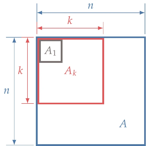
Figure A.9:For to be positive definite, the determinants of the submatrices must be greater than zero.
Another practical condition equivalent to Equation A.42 is that all the leading principal minors of are positive. A leading principal minor is the determinant of a leading principal submatrix. A leading principal submatrix of order , of an matrix is obtained by removing the last rows and columns of , as shown in Figure A.9. Thus, to verify if is positive definite, we start with , check that (only one element), then check that , and so on, until . Suppose any of the determinants in this sequence is not positive. In that case, we can stop the process and conclude that is not positive definite.
A positive-semidefinite matrix satisfies
for all nonzero vectors . In this case, the eigenvalues are nonnegative, and there is at least one that is zero. A negative-definite matrix satisfies
for all nonzero vectors . In this case, all the eigenvalues are negative. An indefinite matrix is one that is neither positive definite nor negative definite. Then, there are at least two nonzero vectors and such that
A.7 Matrix Derivatives
Let us consider the derivatives of a few common cases: linear and quadratic functions. Combining the concept of partial derivatives and matrix forms of equations allows us to find the gradients of matrix functions. First, let us consider a linear function, , defined as
where , , and are vectors of length , and are the th elements of , respectively. If we take the partial derivative of each element with respect to an arbitrary element of , namely, , we get
Thus,
Recall the quadratic form presented in Section A.3.3; we can combine that with a linear term to form a general quadratic function:
where , and are still vectors of length , and is an -by- symmetric matrix. In index notation, is as follows:
For convenience, we separate the diagonal terms from the off-diagonal terms, leaving us with
Now we take the partial derivatives with respect to as before, yielding
We now move the diagonal terms back into the sums to get
which we can put back into matrix form as follows:
If is symmetric, then , and thus
A.8 Eigenvalues and Eigenvectors
Given an matrix, if there is a scalar and a nonzero vector that satisfy
then is an eigenvalue of the matrix , and is an eigenvector.
The left-hand side of Equation A.57 is a matrix-vector product that represents a linear transformation applied to . The right-hand side of Equation A.57 is a scalar-vector product that represents a vector aligned with . Therefore, the eigenvalue problem (Equation A.57) answers the question: Which vectors, when transformed by , remain in the same direction, and how much do their corresponding lengths change in that transformation?
The solutions of the eigenvalue problem (Equation A.57) are given by the solutions of the scalar equation,
This equation yields a polynomial of degree called the characteristic equation, whose roots are the eigenvalues of .
If is symmetric, it has real eigenvalues and linearly independent eigenvectors corresponding to those eigenvalues. It is possible to choose the eigenvectors to be orthogonal to each other (i.e., for ) and to normalize them (so that ).
We use the eigenvalue problem in Section 4.1.2, where the eigenvectors are the directions of principal curvature, and the eigenvalues quantify the curvature. Eigenvalues are also helpful in determining if a matrix is positive definite.
A.9 Random Variables
Imagine measuring the axial strength of a rod by performing a tensile test with many rods, each designed to be identical. Even with “identical” rods, every time you perform the test, you get a different result (hopefully with relatively small differences). This variation has many potential sources, including variation in the manufactured size and shape, in the composition of the material, and in the contact between the rod and testing fixture. In this example, we would call the axial strength a random variable, and the result from one test would be a random sample. The random variable, axial strength, is a function of several other random variables, such as bar length, bar diameter, and material Young’s modulus.
One measurement does not tell us anything about how variable the axial strength is, but if we perform the test many times, we can learn a lot about its distribution. From this information, we can infer various statistical quantities, such as the mean value of the axial strength. The mean of some variable that is measured times is estimated as follows:
This is actually a sample mean, which would differ from the population mean (the true mean if you could measure every bar). With enough samples, the sample mean approaches the population mean. In this brief review, we do not distinguish between sample and population statistics.
Another important quantity is the variance or standard deviation. This is a measure of spread, or how far away our samples are from the mean. The unbiased[3]estimate of the variance is
and the standard deviation is just the square root of the variance. A small variance implies that measurements are clustered tightly around the mean, whereas a large variance means that measurements are spread out far from the mean. The variance can also be written in the following mathematically equivalent but more computationally-friendly format:
More generally, we might want to know what the probability is of getting a bar with a specific axial strength. In our testing, we could tabulate the frequency of each measurement in a histogram. If done enough times, it would define a smooth curve, as shown in Figure A.10. This curve is called the probability density function (PDF), , and it tells us the relative probability of a certain value occurring.
More specifically, a PDF gives the probability of getting a value with a certain range:
The total integral of the PDF must be 1 because it contains all possible outcomes (100 percent):
From the PDF, we can also measure various statistics, such as the mean value:
This quantity is also referred to as the expected value of (). The expected value of a function of a random variable, , is given by:[4]
We can also compute the variance, which is the expected value of the squared difference from the mean:
or in a mathematically equivalent format:
The mean and variance are the first and second moments of the distribution. In general, a distribution may require an infinite number of moments to describe it fully. Higher-order moments are generally mean centered and are normalized by the standard deviation so that the th normalized moment is computed as follows:
The third moment is called skewness, and the fourth is called kurtosis, although these higher-order moments are less commonly used.
The cumulative distribution function (CDF) is related to the PDF, which is the cumulative integral of the PDF and is defined as follows:
The capital denotes the CDF, and the lowercase denotes the PDF. As an example, the PDF and corresponding CDF for the axial strength are shown in Figure A.10. The CDF always approaches 1 as .
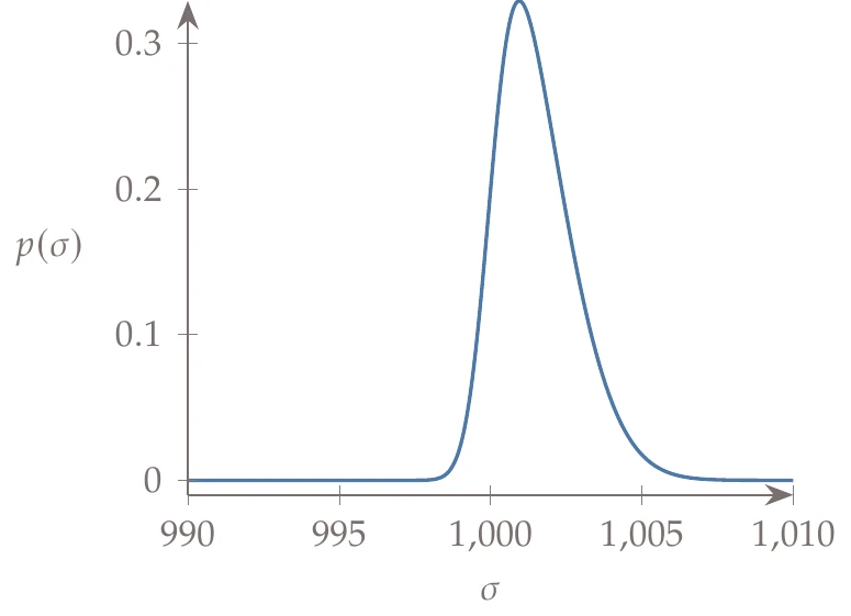
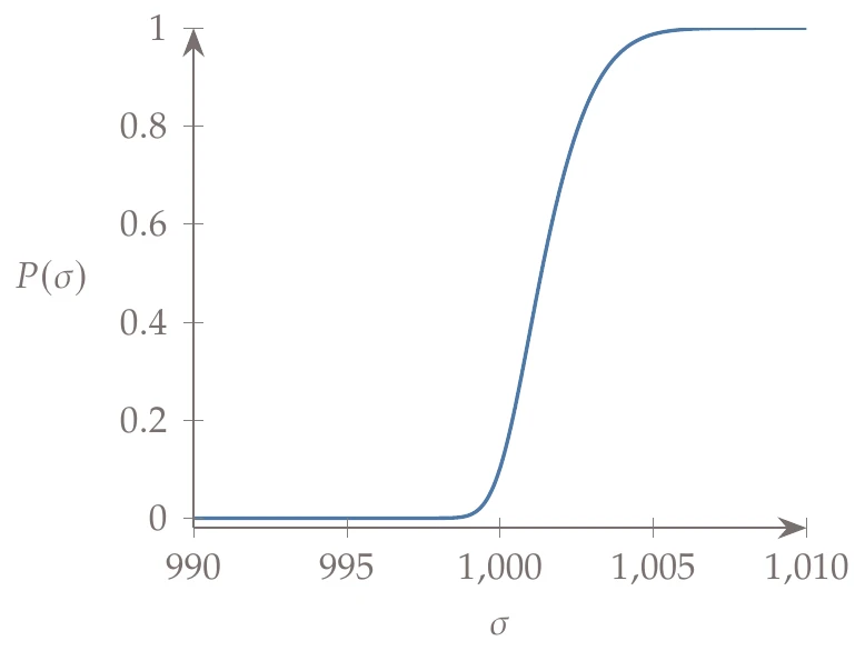
Figure A.10:Comparison between PDF and CDF for a simple example.
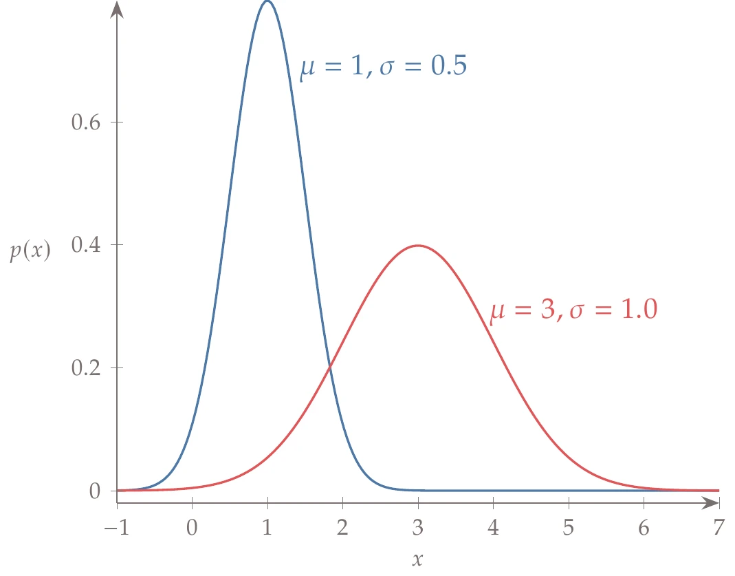
Figure A.11:Two normal distributions. Changing the mean causes a shift along the -axis. Increasing the standard deviation causes the PDF to spread out.
We often fit a named distribution to the PDF of empirical data. One of the most popular distributions is the normal distribution, also known as the Gaussian distribution. Its PDF is as follows:
For a normal distribution, the mean and variance are visible in the function, but these quantities are defined for any distribution. Figure A.11 shows two normal distributions with different means and standard deviations to illustrate the effect of those parameters.
Several other popular distributions are shown in Figure A.12: uniform distribution, Weibull distribution, lognormal distribution, and exponential distribution. These are only a few of many other possible probability distributions.
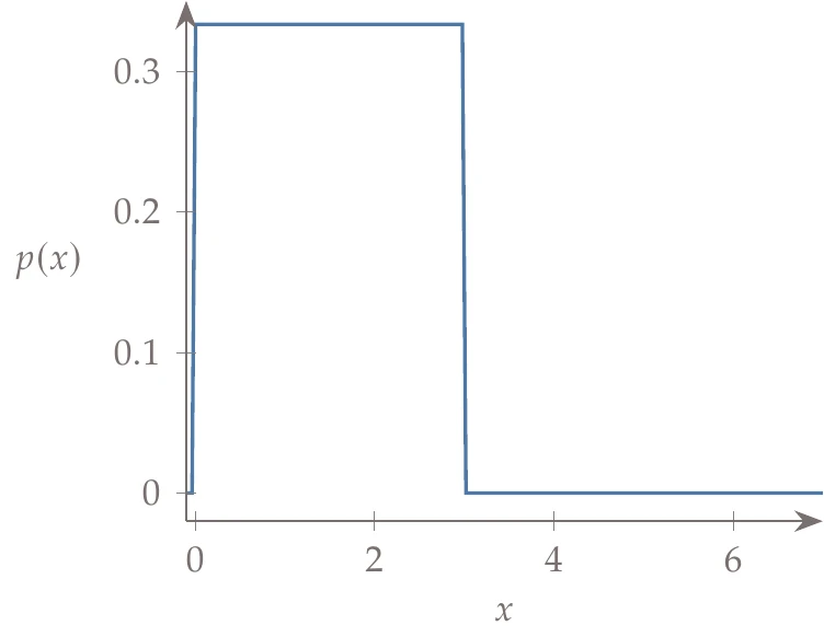
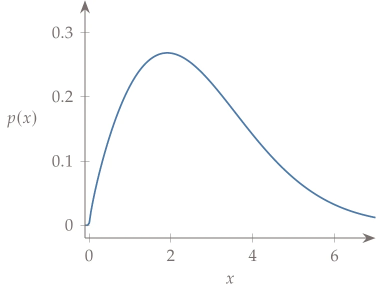
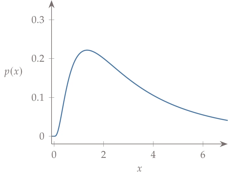
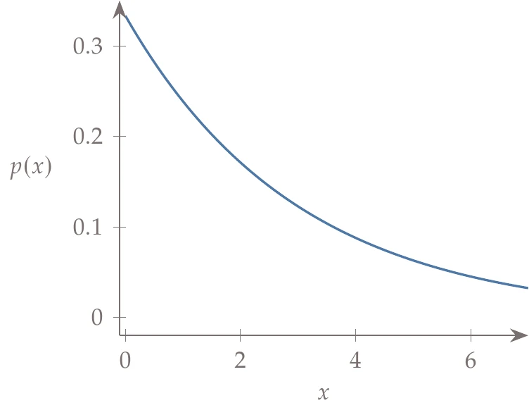
Figure A.12a:Popular probability distributions besides the normal distribution.
An extension of variance is the covariance, which measures the variability between two random variables:
From this definition, we see that the variance is related to covariance by the following:
Covariance is often expressed as a matrix, in which case the variance of each variable appears on the diagonal. The correlation is the covariance divided by the standard deviations:
In this notation, is the number of rows and is the number of columns.
1 provides a comprehensive coverage of linear algebra and is credited with popularizing the concept of the “four fundamental subspaces”.
Unbiased means that the expected value of the sample variance is the same as the true population variance. If were used in the denominator instead of , then the two quantities would differ by a constant.
This is not a definition, but rather uses the expected value definition with a somewhat lengthy derivation.
- Strang, G. (2006). Linear Algebra and its Applications (4th ed.). Cengage Learning.