6 Computing Derivatives
The gradient-based optimization methods introduced in Chapter 4 and Chapter 5 require the derivatives of the objective and constraints with respect to the design variables, as illustrated in Figure 6.1. Derivatives also play a central role in other numerical algorithms. For example, the Newton-based methods introduced in Section 3.8 require the derivatives of the residuals.
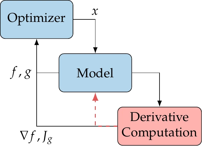
Figure 6.1:Efficient derivative computation is crucial for the overall efficiency of gradient-based optimization.
The accuracy and computational cost of the derivatives are critical for the success of these methods. Gradient-based methods are only efficient when the derivative computation is also efficient. The computation of derivatives can be the bottleneck in the overall optimization procedure, especially when the model solver needs to be called repeatedly. This chapter introduces the various methods for computing derivatives and discusses the relative advantages of each method.
6.1 Derivatives, Gradients, and Jacobians
The derivatives we focus on are first-order derivatives of one or more functions of interest () with respect to a vector of variables (). In the engineering optimization literature, the term sensitivity analysis is often used to refer to the computation of derivatives, and derivatives are sometimes referred to as sensitivity derivatives or design sensitivities. Although these terms are not incorrect, we prefer to use the more specific and concise term derivative.
For the sake of generality, we do not specify which functions we want to differentiate in this chapter (which could be an objective, constraints, residuals, or any other function). Instead, we refer to the functions being differentiated as the functions of interest and represent them as a vector-valued function, . Neither do we specify the variables with respect to which we differentiate (which could be design variables, state variables, or any other independent variable).
The derivatives of all the functions of interest with respect to all the variables form a Jacobian matrix,
which is an rectangular matrix where each row corresponds to the gradient of each function with respect to all the variables.
Row of the Jacobian is the gradient of function . Each column in the Jacobian is called the tangent with respect to a given variable . The Jacobian can be related to the operator as follows:
6.2 Overview of Methods for Computing Derivatives
We can classify the methods for computing derivatives according to the representation used for the numerical model. There are three possible representations, as shown in Figure 6.2. In one extreme, we know nothing about the model and consider it a black box where we can only control the inputs and observe the outputs (Figure 6.2, left). In this chapter, we often refer to as the input variables and as the output variables. When this is the case, we can only compute derivatives using finite differences (Section 6.4).
In the other extreme, we have access to the source code used to compute the functions of interest and perform the differentiation line by line (Figure 6.2, right). This is the essence of the algorithmic differentiation approach (Section 6.6). The complex-step method (Section 6.5) is related to algorithmic differentiation, as explained in Section 6.6.5.
In the intermediate case, we consider the model residuals and states (Figure 6.2, middle), which are the quantities required to derive and implement implicit analytic methods (Section 6.7). When the model can be represented with multiple components, we can use a coupled derivative approach (Section 13.3) where any of these derivative computation methods can be used for each component.

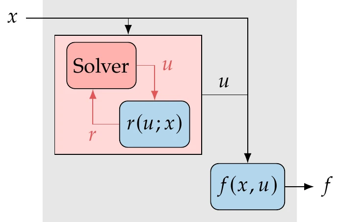
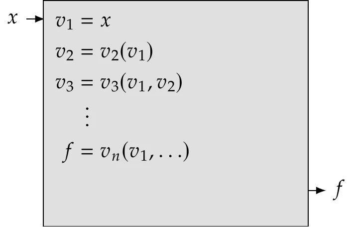
Figure 6.2:Derivative computation methods can consider three different levels of information: function values (a), model states (b), and lines of code (c).
6.3 Symbolic Differentiation
Symbolic differentiation is well known and widely used in calculus, but it is of limited use in the numerical optimization of most engineering models. Except for the most straightforward cases (e.g., Example 6.1), many engineering models involve a large number of operations, utilize loops and various conditional logic, are implicitly defined, or involve iterative solvers (see Chapter 3). Although the mathematical expressions within these iterative procedures is explicit, it is challenging, or even impossible, to use symbolic differentiation to obtain closed-form mathematical expressions for the derivatives of the procedure. Even when it is possible, these expressions are almost always computationally inefficient.
Symbolic differentiation is still valuable for obtaining derivatives of simple explicit components within a larger model. Furthermore, algorithm differentiation (discussed in a later section) relies on symbolic differentiation to differentiate each line of code in the model.
6.4 Finite Differences
Because of their simplicity, finite-difference methods are a popular approach to computing derivatives. They are versatile, requiring nothing more than function values. Finite differences are the only viable option when we are dealing with black-box functions because they do not require any knowledge about how the function is evaluated. Most gradient-based optimization algorithms perform finite differences by default when the user does not provide the required gradients. However, finite differences are neither accurate nor efficient.
6.4.1 Finite-Difference Formulas
Finite-difference approximations are derived by combining Taylor series expansions. It is possible to obtain finite-difference formulas that estimate an arbitrary order derivative with any order of truncation error by using the right combinations of these expansions. The simplest finite-difference formula can be derived directly from a Taylor series expansion in the direction,
where is the unit vector in the direction. Solving this for the first derivative, we obtain the finite-difference formula,
where is a small scalar called the finite-difference step size.
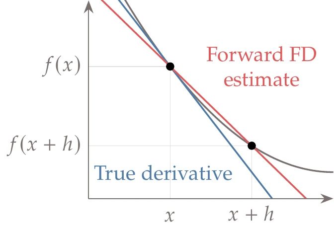
Figure 6.3:Exact derivative compared with a forward finite-difference approximation (Equation 6.4).
This approximation is called the forward difference and is directly related to the definition of a derivative because
The truncation error is , and therefore this is a first-order approximation. The difference between this approximation and the exact derivative is illustrated in Figure 6.3.
The backward-difference approximation can be obtained by replacing with to yield
which is also a first-order approximation.
Assuming each function evaluation yields the full vector , the previous formulas compute the column of the Jacobian in Equation 6.1. To compute the full Jacobian, we need to loop through each direction , add a step, recompute , and compute a finite difference. Hence, the cost of computing the complete Jacobian is proportional to the number of input variables of interest, .
For a second-order estimate of the first derivative, we can use the expansion of to obtain
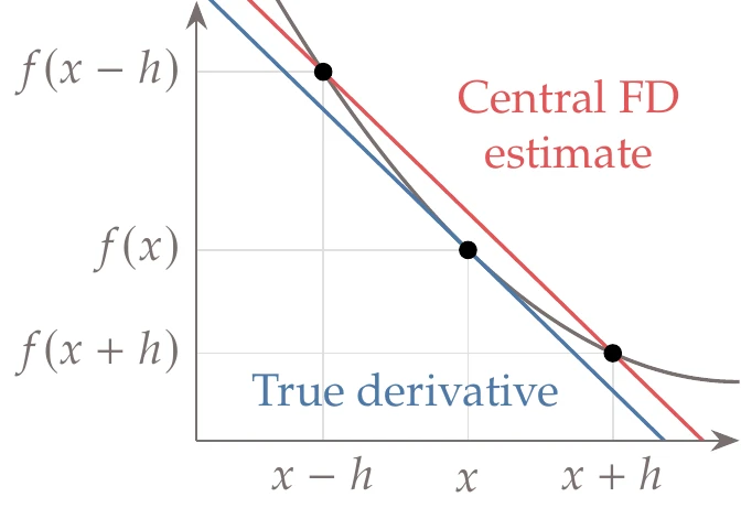
Figure 6.4:Exact derivative compared with a central finite-difference approximation (Equation 6.8).
Then, if we subtract this from the expansion in Equation 6.3 and solve the resulting equation for the derivative of , we get the central-difference formula,
The stencil of points for this formula is shown in Figure 6.4, where we can see that this estimate is closer to the actual derivative than the forward difference.
Even more accurate estimates can be derived by combining different Taylor series expansions to obtain higher-order truncation error terms. This technique is widely used in finite-difference methods for solving differential equations, where higher-order estimates are desirable.
However, finite-precision arithmetic eventually limits the achievable accuracy for our purposes (as discussed in the next section). With double-precision arithmetic, there are not enough significant digits to realize a significant advantage beyond central difference.
We can also estimate second derivatives (or higher) by combining Taylor series expansions. For example, adding the expansions for and cancels out the first derivative and third derivative terms, yielding the second-order approximation to the second-order derivative,
The finite-difference method can also be used to compute directional derivatives, which are the scalar projection of the gradient into a given direction. To do this, instead of stepping in orthogonal directions to get the gradient, we need to step in the direction of interest, , as shown in Figure 6.5. Using the forward difference, for example,
One application of directional derivatives is to compute the slope in line searches (Section 4.3).
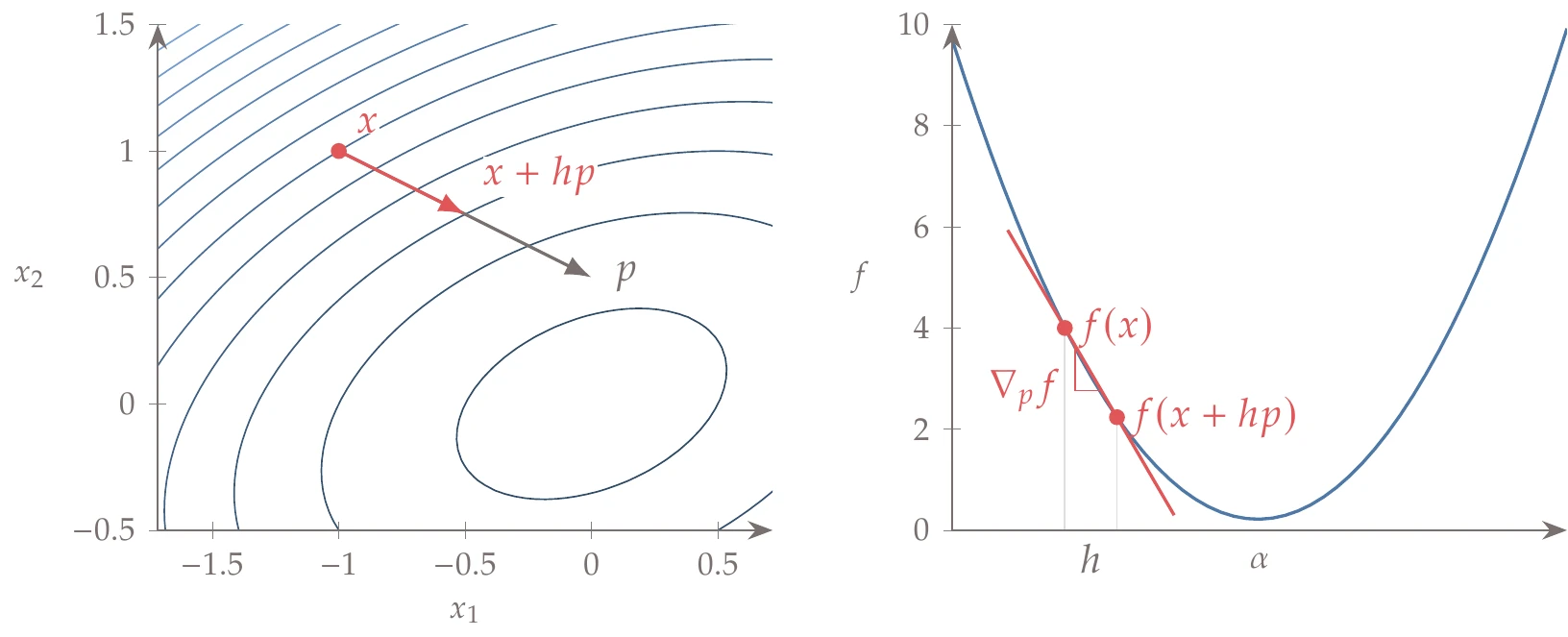
Figure 6.5:Computing a directional derivative using a forward finite difference.
6.4.2 The Step-Size Dilemma
When estimating derivatives using finite-difference formulas, we are faced with the step-size dilemma. Because each estimate has a truncation error of (or when second order), we would like to choose as small of a step size as possible to reduce this error. However, as the step size reduces, subtractive cancellation (a roundoff error introduced in Section 3.5.1) becomes dominant. Given the opposing trends of these errors, there is an optimal step size for which the sum of the two errors is at a minimum.
Theoretically, the optimal step size for the forward finite difference is approximately , where is the precision of . The error bound is also about . For the central difference, the optimal step size scales approximately with , with an error bound of . These step and error bound estimates are just approximate and assume well-scaled problems.
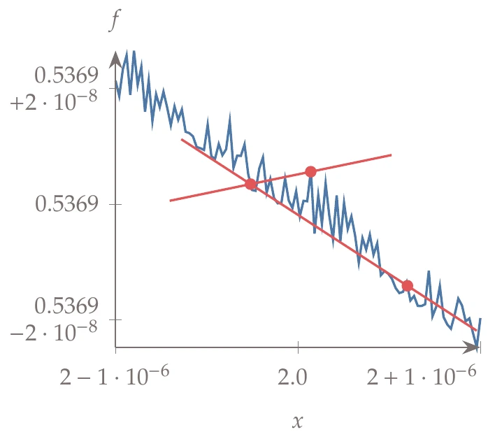
Figure 6.8:Finite-differencing noisy functions can either smooth the derivative estimates or result in estimates with the wrong trends.
Finite-difference approximations are sometimes used with larger steps than would be desirable from an accuracy standpoint to help smooth out numerical noise or discontinuities in the model. This approach sometimes works, but it is better to address these problems within the model whenever possible. Figure 6.8 shows an example of this effect. For this noisy function, the larger step ignores the noise and gives the correct trend, whereas the smaller step results in an estimate with the wrong sign.
6.4.3 Practical Implementation
Algorithm 6.1 details a procedure for computing a Jacobian using forward finite differences. It is usually helpful to scale the step size based on the value of , unless is too small. Therefore, we combine the relative and absolute quantities to obtain the following step size:
This is similar to the expression for the convergence criterion in Equation 4.24. Although the absolute step size usually differs for each , the relative step size is often the same and is user-specified.
6.5 Complex Step
The complex-step derivative approximation, strangely enough, computes derivatives of real functions using complex variables. Unlike finite differences, the complex-step method requires access to the source code and cannot be applied to black-box components. The complex-step method is accurate but no more efficient than finite differences because the computational cost still scales linearly with the number of variables.
6.5.1 Theory
The complex-step method can also be derived using a Taylor series expansion. Rather than using a real step , as we did to derive the finite-difference formulas, we use a pure imaginary step, .[2] If is a real function in real variables and is also analytic (differentiable in the complex domain), we can expand it in a Taylor series about a real point as follows:
Taking the imaginary parts of both sides of this equation, we have
Dividing this by and solving for yields the complex-step derivative approximation,[3]
which is a second-order approximation. To use this approximation, we must provide a complex number with a perturbation in the imaginary part, compute the original function using complex arithmetic, and take the imaginary part of the output to obtain the derivative.
In practical terms, this means that we must convert the function evaluation to take complex numbers as inputs and compute complex outputs. Because we have assumed that is a real function of a real variable in the derivation of Equation 6.14, the procedure described here does not work for models that already involve complex arithmetic.
In Section 6.5.2, we explain how to convert programs to handle the required complex arithmetic for the complex-step method to work in general. The complex-step method has been extended to compute exact second derivatives as well.45
Unlike finite differences, this formula has no subtraction operation and thus no subtractive cancellation error. The only source of numerical error is the truncation error. However, the truncation error can be eliminated if is decreased to a small enough value (say, 10-200). Then, the precision of the complex-step derivative approximation (Equation 6.14) matches the precision of . This is a tremendous advantage over the finite-difference approximations (Equation 6.4 and Equation 6.8).
Like the finite-difference approach, each evaluation yields a column of the Jacobian (), and the cost of computing all the derivatives is proportional to the number of design variables. The cost of the complex-step method is comparable to that of a central difference because we compute a real and an imaginary part for every number in our code.
If we take the real part of the Taylor series expansion (Equation 6.12), we obtain the value of the function on the real axis,
Similar to the derivative approximation, we can make the truncation error disappear by using a small enough . This means that no separate evaluation of is required to get the original real value of the function; we can simply take the real part of the complex evaluation.
What is a “small enough ”? When working with finite-precision arithmetic, the error can be eliminated entirely by choosing an so small that all terms become zero because of underflow (i.e., is smaller than the smallest representable number, which is approximately 10-324 when using double precision; see Section 3.5.1). Eliminating these squared terms does not affect the accuracy of the derivative carried in the imaginary part because the squared terms only appear in the error terms of the complex-step approximation.
At the same time, must be large enough that the imaginary part () does not underflow.
Suppose that is the smallest representable number. Then, the two requirements result in the following bounds:
A step size of 10-200 works well for double-precision functions.
6.5.2 Complex-Step Implementation
We can use the complex-step method even when the evaluation of involves the solution of numerical models through computer programs.3 The outer loop for computing the derivatives of multiple functions with respect to all variables (Algorithm 6.2) is similar to the one for finite differences. A reference function evaluation is not required, but now the function must handle complex numbers correctly.
The complex-step method can be applied to any model, but modifications might be required. We need the source code for the model to make sure that the program can handle complex numbers and the associated arithmetic, that it handles logical operators consistently, and that certain functions yield the correct derivatives.
First, the program may need to be modified to use complex numbers. In programming languages like Fortran or C, this involves changing real-valued type declarations (e.g., double) to complex type declarations (e.g., double complex). In some languages, such as MATLAB, Python, and Julia, this is unnecessary because functions are overloaded to automatically accept either type.
Second, some changes may be required to preserve the correct logical flow through the program. Relational logic operators (e.g., “greater than”, “less than”, “if”, and “else”) are usually not defined for complex numbers. These operators are often used in programs, together with conditional statements, to redirect the execution thread. The original algorithm and its “complexified” version should follow the same execution thread. Therefore, defining these operators to compare only the real parts of the arguments is the correct approach. Functions that choose one argument, such as the maximum or the minimum values, are based on relational operators. Following the previous argument, we should determine the maximum and minimum values based on the real parts alone.
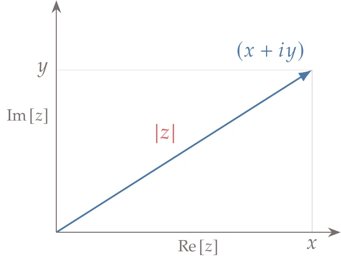
Figure 6.10:The usual definition of a complex absolute value returns a real number (the length of the vector), which is not compatible with the complex-step method.
Third, some functions need to be redefined for complex arguments. The most common function that needs to be redefined is the absolute value function. For a complex number, , the absolute value is defined as
as shown in Figure 6.10. This definition is not complex analytic, which is required in the derivation of the complex-step derivative approximation.
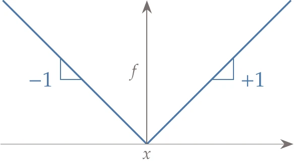
Figure 6.11:The absolute value function needs to be redefined such that the imaginary part yields the correct derivatives.
As shown in Figure 6.11, the correct derivatives for the real absolute value function are +1 and -1, depending on whether is greater than or less than zero. The following complex definition of the absolute value yields the correct derivatives:
Setting the imaginary part to and dividing by corresponds to the slope of the absolute value function. There is an exception at , where the function is not analytic, but a derivative does not exist in any case. We use the “greater or equal” in the logic so that the approximation yields the correct right-sided derivative at that point.
Depending on the programming language, we may need to redefine some trigonometric functions. This is because some default implementations, although correct, do not maintain accurate derivatives for small complex-step sizes.
We must replace these with mathematically equivalent implementations that avoid numerical issues.
Fortunately, we can automate most of these changes by using scripts to process the codes, and in most programming languages, we can easily redefine functions using operator overloading.[4]
6.6 Algorithmic Differentiation
Algorithmic differentiation (AD)—also known as computational differentiation or automatic differentiation—is a well-known approach based on the systematic application of the chain rule to computer programs.67 The derivatives computed with AD can match the precision of the function evaluation.
The cost of computing derivatives with AD can be proportional to either the number of variables or the number of functions, depending on the type of AD, making it flexible.
Another attractive feature of AD is that its implementation is largely automatic, thanks to various AD tools. To explain AD, we start by outlining the basic theory with simple examples. Then we explore how the method is implemented in practice with further examples.
6.6.1 Variables and Functions as Lines of Code
The basic concept of AD is as follows. Even long, complicated codes consist of a sequence of basic operations (e.g., addition, multiplication, cosine, exponentiation). Each operation can be differentiated symbolically with respect to the variables in the expression.
AD performs this symbolic differentiation and adds the code that computes the derivatives for each variable in the code. The derivatives of each variable accumulate in what amounts to a numerical version of the chain rule.
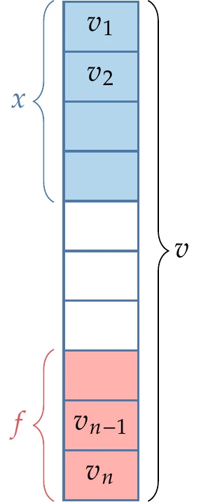
Figure 6.13:AD considers all the variables in the code, where the inputs are among the first variables, and the outputs are among the last.
The fundamental building blocks of a code are unary and binary operations. These operations can be combined to obtain more elaborate explicit functions, which are typically expressed in one line of computer code. We represent the variables in the computer code as the sequence , where is the total number of variables assigned in the code. One or more of these variables at the start of this sequence are given and correspond to , and one or more of the variables toward the end of the sequence are the outputs of interest, , as illustrated in Figure 6.13.
In general, a variable assignment corresponding to a line of code can involve any other variable, including itself, through an explicit function,
Except for the most straightforward codes, many of the variables in the code are overwritten as a result of iterative loops.
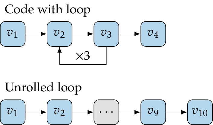
Figure 6.14:Unrolling of loops is a useful mental model to understand the derivative propagation in the AD of general code.
To understand AD, it is helpful to imagine a version of the code where all the loops are unrolled. Instead of overwriting variables, we create new versions of those variables, as illustrated in Figure 6.14. Then, we can represent the computations in the code in a sequence with no loops such that each variable in this larger set only depends on previous variables, and then
Given such a sequence of operations and the derivatives for each operation, we can apply the chain rule to obtain the derivatives for the entire sequence. Unrolling the loops is just a mental model for understanding how the chain rule operates, and it is not explicitly done in practice.
The chain rule can be applied in two ways. In the forward mode, we choose one input variable and work forward toward the outputs until we get the desired total derivative. In the reverse mode, we choose one output variable and work backward toward the inputs until we get the desired total derivative.
6.6.2 Forward-Mode AD
The chain rule for the forward mode can be written as
where each partial derivative is obtained by symbolically differentiating the explicit expression for . The total derivatives are the derivatives with respect to the chosen input , which can be computed using this chain rule.
Using the forward mode, we evaluate a sequence of these expressions by fixing in Equation 6.21 (effectively choosing one input ) and incrementing to get the derivative of each variable . We only need to sum up to because of the form of Equation 6.20, where each only depends on variables that precede it.
For a more convenient notation, we define a new variable that represents the total derivative of variable with respect to a fixed input as and rewrite the chain rule as
The chosen input corresponds to the seed, which we set to (using the definition for , we see that means setting ).
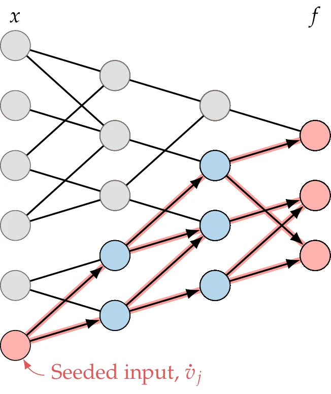
Figure 6.15:The forward mode propagates derivatives to all the variables that depend on the seeded input variable.
This chain rule then propagates the total derivatives forward, as shown in Figure 6.15, affecting all the variables that depend on the seeded variable.
Once we are done applying the chain rule (Equation 6.22) for the chosen input variable , we end up with the total derivatives for all . The sum in the chain rule (Equation 6.22) only needs to consider the nonzero partial derivative terms. If a variable does not explicitly appear in the expression for , then , and there is no need to consider the corresponding term in the sum. In practice, this means that only a small number of terms is considered for each sum.
Suppose we have four variables , and , and , , and we want . We assume that each variable depends explicitly on all the previous ones. Using the chain rule (Equation 6.22), we set (because we want the derivative with respect to ) and increment in to get the sequence of derivatives:
In each step, we just need to compute the partial derivatives of the current operation and then multiply using the total derivatives that have already been computed. We move forward by evaluating the partial derivatives of in the same sequence to evaluate the original function.
This is convenient because all of the unknowns are partial derivatives, meaning that we only need to compute derivatives based on the operation at hand (or line of code).
In this abstract example with four variables that depend on each other sequentially, the Jacobian of the variables with respect to themselves is as follows:
By setting the seed and using the forward chain rule (Equation 6.22), we have computed the first column of from top to bottom. This column corresponds to the tangent with respect to . Using forward-mode AD, obtaining derivatives for other outputs is free (e.g., in Equation 6.23).
However, if we want the derivatives with respect to additional inputs, we would need to set a different seed and evaluate an entire set of similar calculations. For example, if we wanted , we would set the seed as and evaluate the equations for and , where we would now have . This would correspond to computing the second column in (Equation 6.24).
Thus, the cost of the forward mode scales linearly with the number of inputs we are interested in and is independent of the number of outputs.
So far, we have assumed that we are computing derivatives with respect to each component of . However, just like for finite differences, we can also compute directional derivatives using forward-mode AD. We do so by setting the appropriate seed in the ’s that correspond to the inputs in a vectorized manner. Suppose we have . To compute the derivative with respect to , we would set the seed as the unit vector and follow a similar process for the other elements. To compute a directional derivative in direction , we would set the seed as .
6.6.3 Reverse-Mode AD
The reverse mode is also based on the chain rule but uses the alternative form:
where the summation happens in reverse (starts at and decrements to ). This is less intuitive than the forward chain rule, but it is equally valid. Here, we fix the index corresponding to the output of interest and decrement until we get the desired derivative.
Similar to the forward-mode total derivative notation (Equation 6.22), we define a more convenient notation for the variables that carry the total derivatives with a fixed as ,
which are sometimes called adjoint variables. Then we can rewrite the chain rule as
This chain rule propagates the total derivatives backward after setting the reverse seed , as shown in Figure 6.18.
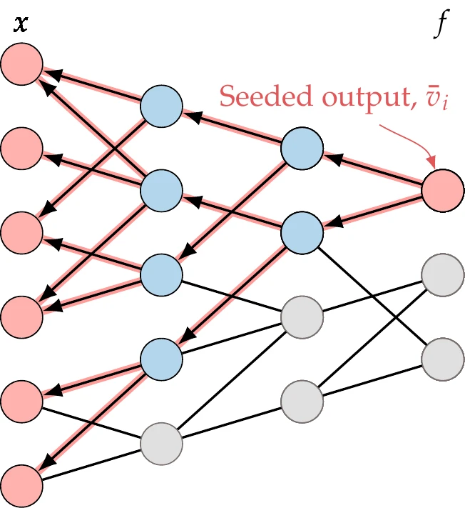
Figure 6.18:The reverse mode propagates derivatives to all the variables on which the seeded output variable depends.
This affects all the variables on which the seeded variable depends.
The reverse-mode variables represent the derivatives of one output, , with respect to all the input variables (instead of the derivatives of all the outputs with respect to one input, , in the forward mode). Once we are done applying the reverse chain rule (Equation 6.27) for the chosen output variable , we end up with the total derivatives for all .
Applying the reverse mode to the same four-variable example as before, we get the following sequence of derivative computations (we set and decrement ):
The partial derivatives of must be computed for first, then , and so on. Therefore, we have to traverse the code in reverse. In practice, not every variable depends on every other variable, so a computational graph is created during code evaluation. Then, when computing the adjoint variables, we traverse the computational graph in reverse. As before, the derivatives we need to compute in each line are only partial derivatives.
Recall the Jacobian of the variables,
By setting and using the reverse chain rule (Equation 6.27), we have computed the last row of from right to left. This row corresponds to the gradient of . Using the reverse mode of AD, obtaining derivatives with respect to additional inputs is free (e.g., in Equation 6.28).
However, if we wanted the derivatives of additional outputs, we would need to evaluate a different sequence of derivatives. For example, if we wanted , we would set and evaluate the expressions for and in Equation 6.28, where . Thus, the cost of the reverse mode scales linearly with the number of outputs and is independent of the number of inputs.
One complication with the reverse mode is that the resulting sequence of derivatives requires the values of the variables, starting with the last ones and progressing in reverse. For example, the partial derivative in the second operation of Equation 6.28 might involve . Therefore, the code needs to run in a forward pass first, and all the variables must be stored for use in the reverse pass, which increases memory usage.
Unlike with forward-mode AD and finite differences, it is impossible to compute a directional derivative by setting the appropriate seeds.
Although the seeds in the forward mode are associated with the inputs, the seeds for the reverse mode are associated with the outputs. Suppose we have multiple functions of interest, . To find the derivatives of in a vectorized operation, we would set .
A seed with multiple nonzero elements computes the derivatives of a weighted function with respect to all the variables, where the weight for each function is determined by the corresponding value.
6.6.4 Forward Mode or Reverse Mode?
Our goal is to compute , the () matrix of derivatives of all the functions of interest with respect to all the input variables . However, AD computes many other derivatives corresponding to intermediate variables. The complete Jacobian for all the intermediate variables, , assuming that the loops have been unrolled, has the structure shown in Figure 6.22 and Figure 6.23.
The input variables are among the first entries in , whereas the functions of interest are among the last entries of .
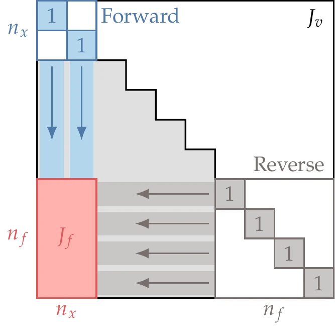
Figure 6.22:When , the forward mode is advantageous.
For simplicity, let us assume that the entries corresponding to and are contiguous, as previously shown in Figure 6.13. Then, the derivatives we want () are a block located on the lower left in the much larger matrix (), as shown in Figure 6.22 and Figure 6.23. Although we are only interested in this block, AD requires the computation of additional intermediate derivatives.
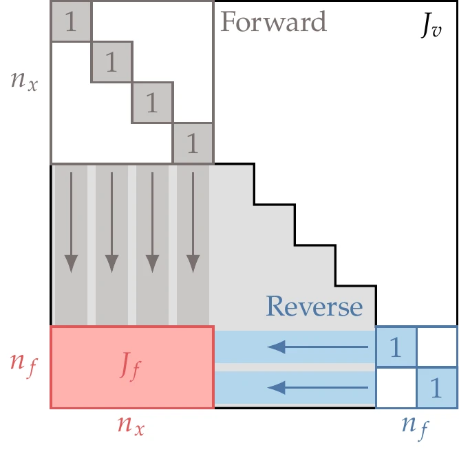
Figure 6.23:When , the reverse mode is advantageous.
The main difference between the forward and the reverse approaches is that the forward mode computes the Jacobian column by column, whereas the reverse mode does it row by row. Thus, the cost of the forward mode is proportional to , whereas the cost of the reverse mode is proportional to . If we have more outputs (e.g., objective and constraints) than inputs (design variables), the forward mode is more efficient, as illustrated in Figure 6.22. On the other hand, if we have many more inputs than outputs, then the reverse mode is more efficient, as illustrated in Figure 6.23. If the number of inputs is similar to the number of outputs, neither mode has a significant advantage.
In both modes, each forward or reverse pass costs less than 2–3 times the cost of running the original code in practice. However, because the reverse mode requires storing a large amount of data, memory costs also need to be considered. In principle, the required memory is proportional to the number of variables, but there are techniques that can reduce the memory usage significantly.[5]
6.6.5 AD Implementation
There are two main ways to implement AD: by source code transformation or by operator overloading. The function we used to demonstrate the issues with symbolic differentiation (Example 6.2) can be differentiated much more easily with AD. In the examples that follow, we use this function to demonstrate how the forward and reverse mode work using both source code transformation and operator overloading.
Source Code Transformation
AD tools that use source code transformation process the whole source code automatically with a parser and add lines of code that compute the derivatives. The added code is highlighted in Example 6.7 and Example 6.8.
Operator Overloading
The operator overloading approach creates a new augmented data type that stores both the variable value and its derivative. Every floating-point number is replaced by a new type with two parts , commonly referred to as a dual number. All standard operations (e.g., addition, multiplication, sine) are overloaded such that they compute according to the original function value and according to the derivative of that function. For example, the multiplication operation, , would be defined for the dual-number data type as
where we compute the original function value in the first term, and the second term carries the derivative of the multiplication.
Although we wrote the two parts explicitly in Equation 6.31, the source code would only show a normal multiplication, such as . However, each of these variables would be of the new type and carry the corresponding quantities. By overloading all the required operations, the computations happen “behind the scenes”, and the source code does not have to be changed, except to declare all the variables to be of the new type and to set the seed. Example 6.9 lists the original code from Example 6.2 with notes on the actual computations that are performed as a result of overloading.
The implementation of the reverse mode using operating overloading is less straightforward and is not detailed here. It requires a new data type that stores the information from the computational graph and the variable values when running the forward pass. This information can be stored using the taping technique. After the forward evaluation of using the new type, the “tape” holds the sequence of operations, which is then evaluated in reverse to propagate the reverse-mode seed.[8]
Connection of AD with the Complex-Step Method
The complex-step method from Section 6.5 can be interpreted as forward-mode AD using operator overloading, where the data type is the complex number , and the imaginary part carries the derivative. To see this connection more clearly, let us write the complex multiplication operation as
This equation is similar to the overloaded multiplication (Equation 6.31). The only difference is that the real part includes the term , which corresponds to the second-order error term in Equation 6.15. In this case, the complex part gives the exact derivative, but a second-order error might appear for other operations. As argued before, these errors vanish in finite-precision arithmetic if the complex step is small enough.
Source Code Transformation versus Operator Overloading
The source code transformation and the operator overloading approaches each have their relative advantages and disadvantages. The overloading approach is much more elegant because the original code stays practically the same and can be maintained directly. On the other hand, the source transformation approach enlarges the original code and results in less readable code, making it hard to work with. Still, it is easier to see what operations take place when debugging. Instead of maintaining source code transformed by AD, it is advisable to work with the original source and devise a workflow where the parser is rerun before compiling a new version.
One advantage of the source code transformation approach is that it tends to yield faster code and allows more straightforward compile-time optimizations. The overloading approach requires a language that supports user-defined data types and operator overloading, whereas source transformation does not. Developing a source transformation AD tool is usually more challenging than developing the overloading approach because it requires an elaborate parser that understands the source syntax.
6.6.6 AD Shortcuts for Matrix Operations
The efficiency of AD can be dramatically increased with manually implemented shortcuts. When the code involves matrix operations, manual implementation of a higher-level differentiation of those operations is more efficient than the line-by-line AD implementation. Giles (2008) documents the forward and reverse differentiation of many matrix elementary operations.
For example, suppose that we have a matrix multiplication . Then, the forward mode yields
The idea is to use and from the AD code preceding the operation and then manually implement this formula (bypassing any AD of the code that performs that operation) to obtain , as shown in Figure 6.24. Then we can use to seed the remainder of the AD code.
The reverse mode of the multiplication yields
Similarly, we take from the reverse AD code and implement the formula manually to compute and , which we can use in the remaining AD code in the reverse procedure.
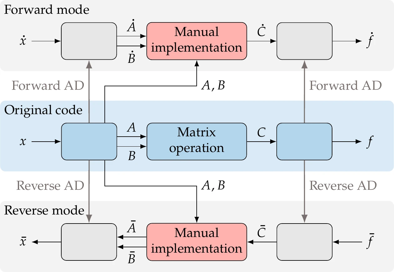
Figure 6.24:Matrix operations, including the solution of linear systems, can be differentiated manually to bypass more costly AD code.
One particularly useful (and astounding!) result is the differentiation of the matrix inverse product. If we have a linear solver such that , we can bypass the solver in the AD process by using the following results:
for the forward mode and
for the reverse mode.
In addition to deriving the formulas just shown, Giles (2008) derives formulas for the matrix derivatives of the inverse, determinant, norms, quadratic, polynomial, exponential, eigenvalues and eigenvectors, and singular value decomposition. Taking shortcuts as described here applies more broadly to any case where a part of the process can be differentiated manually to produce a more efficient derivative computation.
6.7 Implicit Analytic Methods—Direct and Adjoint
Direct and adjoint methods—which we refer to jointly as implicit analytic methods—linearize the model governing equations to obtain a system of linear equations whose solution yields the desired derivatives. Like the complex-step method and AD, implicit analytic methods compute derivatives with a precision matching that of the function evaluation.
The direct method is analogous to forward-mode AD, whereas the adjoint method is analogous to reverse-mode AD.
Analytic methods can be thought of as lying in between the finite-difference method and AD in terms of the number of variables involved. With finite differences, we only need to be aware of inputs and outputs, whereas AD involves every single variable assignment in the code. Analytic methods work at the model level and thus require knowledge of the governing equations and the corresponding state variables.
There are two main approaches to deriving implicit analytic methods: continuous and discrete. The continuous approach linearizes the original continuous governing equations, such as a partial differential equation (PDE), and then discretizes this linearization. The discrete approach linearizes the governing equations only after they have been discretized as a set of residual equations, .
Each approach has its advantages and disadvantages. The discrete approach is preferred and is easier to generalize, so we explain this approach exclusively. One of the primary reasons the discrete approach is preferred is that the resulting derivatives are consistent with the function values because they use the same discretization. The continuous approach is only consistent in the limit of a fine discretization. The resulting inconsistencies can mislead the optimization.[9]
6.7.1 Residuals and Functions
As mentioned in Chapter 3, a discretized numerical model can be written as a system of residuals,
where the semicolon denotes that the design variables are fixed when these equations are solved for the state variables . Through these equations, is an implicit function of . This relationship is represented by the box containing the solver and residual equations in Figure 6.25.
Figure 6.25:Relationship between functions and design variables for a system involving a solver. The implicit equations define the states for a given , so the functions of interest depend explicitly and implicitly on the design variables .
The functions of interest, , are typically explicit functions of the state variables and the design variables. However, because is an implicit function of , is ultimately an implicit function of as well. To compute for a given , we must first find such that . This is usually the most computationally costly step and requires a solver (see Section 3.6). The residual equations could be nonlinear and involve many state variables. In PDE-based models it is common to have millions of states. Once we have solved for the state variables , we can compute the functions of interest . The computation of for a given and is usually much cheaper because it does not require a solver. For example, in PDE-based models, computing such functions typically involves an integration of the states over a surface, or some other transformation of the states.
To compute using finite differences, we would have to use the solver to find for each perturbation of . That means that we would have to run the solver times, which would not scale well when the solution is costly. AD also requires the propagation of derivatives through the solution process. As we will see, implicit analytic methods avoid involving the potentially expensive nonlinear solution in the derivative computation.
6.7.2 Direct and Adjoint Derivative Equations
The derivatives we ultimately want to compute are the ones in the Jacobian . Given the explicit and implicit dependence of on , we can use the chain rule to write the total derivative Jacobian of as
where the result is an matrix.[10]In this context, the total derivatives, , take into account the change in that is required to keep the residuals of the governing equations (Equation 6.37) equal to zero. The partial derivatives in Equation 6.39 represent the variation of with respect to changes in or without regard to satisfying the governing equations.
To better understand the difference between total and partial derivatives in this context, imagine computing these derivatives using finite differences with small perturbations. For the total derivatives, we would perturb , re-solve the governing equations to obtain , and then compute , which would account for both dependency paths in Figure 6.25. To compute the partial derivatives and , however, we would perturb or and recompute without re-solving the governing equations. In general, these partial derivative terms are cheap to compute numerically or can be obtained symbolically.
To find the total derivative , we need to consider the governing equations. Assuming that we are at a point where , any perturbation in must be accompanied by a perturbation in such that the governing equations remain satisfied. Therefore, the differential of the residuals can be written as
This constraint is illustrated in Figure 6.26 in two dimensions, but keep in mind that , , and are vectors in the general case.
The governing equations (Equation 6.37) map an -vector to an -vector . This mapping defines a hypersurface (also known as a manifold) in the – space.
The total derivative that we ultimately want to compute represents the effect that a perturbation on has on subject to the constraint of remaining on this hypersurface, which can be achieved with the appropriate variation in .
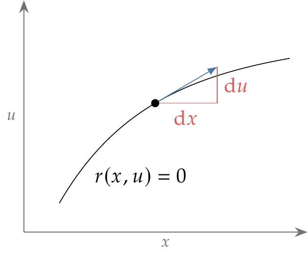
Figure 6.26:The governing equations determine the values of for a given . Given a point that satisfies the equations, the appropriate differential in must accompany a differential of about that point for the equations to remain satisfied.
To obtain a more useful equation, we rearrange Equation 6.40 to get the linear system
where and are both matrices, and is a square matrix of size . This linear system is useful because if we provide the partial derivatives in this equation (which are cheap to compute), we can solve for the total derivatives (whose computation would otherwise require re-solving ). Because is a matrix with columns, this linear system needs to be solved for each with the corresponding column of the right-hand-side matrix .
Now let us assume that we can invert the matrix in the linear system (Equation 6.41) and substitute the solution for into the total derivative equation (Equation 6.39). Then we get
where all the derivative terms on the right-hand side are partial derivatives. The partial derivatives in this equation can be computed using any of the methods that we have described earlier: symbolic differentiation, finite differences, complex step, or AD. Equation 6.42 shows two ways to compute the total derivatives, which we call the direct method and the adjoint method.
The direct method (already outlined earlier) consists of solving the linear system (Equation 6.41) and substituting into Equation 6.39. Defining , we can rewrite Equation 6.41 as
After solving for (one column at the time), we can use it in the total derivative equation (Equation 6.39) to obtain,
This is sometimes called the forward mode because it is analogous to forward-mode AD.
Solving the linear system (Equation 6.43) is typically the most computationally expensive operation in this procedure. The cost of this approach scales with the number of inputs but is essentially independent of the number of outputs . This is the same scaling behavior as finite differences and forward-mode AD. However, the constant of proportionality is typically much smaller in the direct method because we only need to solve the nonlinear equations once to obtain the states.
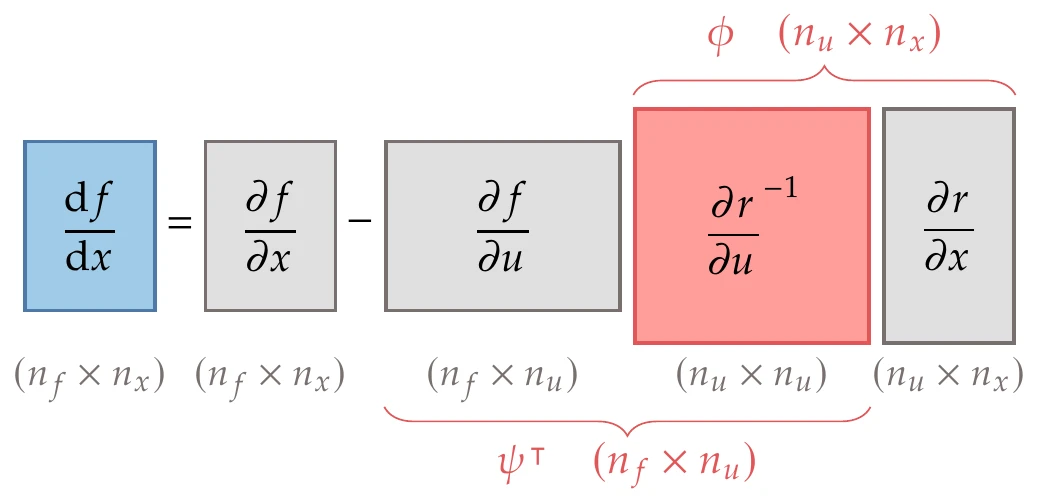
Figure 6.27:The total derivatives (Equation 6.42) can be computed either by solving for (direct method) or by solving for (adjoint method).
The adjoint method changes the linear system that is solved to compute the total derivatives. Looking at Figure 6.27, we see that instead of solving the linear system with on the right-hand side, we can solve it with on the right-hand side. This corresponds to replacing the two Jacobians in the middle with a new matrix of unknowns,
where the columns of are called the adjoint vectors. Multiplying both sides of Equation 6.45 by on the right and taking the transpose of the whole equation, we obtain the adjoint equation,
This linear system has no dependence on . Each adjoint vector is associated with a function of interest and is found by solving the adjoint equation (Equation 6.46) with the corresponding row . The solution () is then used to compute the total derivative
This is sometimes called the reverse mode because it is analogous to reverse-mode AD.
As we will see in Section 6.9, the adjoint vectors are equivalent to the total derivatives , which quantify the change in the function of interest given a perturbation in the residual that gets zeroed out by an appropriate change in .[11]
6.7.3 Direct or Adjoint?
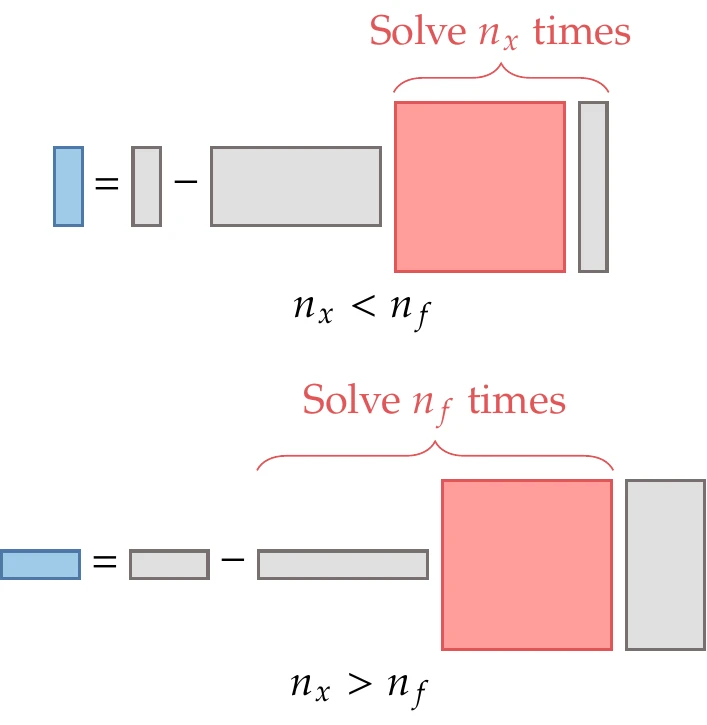
Figure 6.28:Two possibilities for the size of in Figure 6.27. When , it is advantageous to solve the linear system with the vector to the right of the square matrix because it has fewer columns. When , it is advantageous to solve the transposed linear system with the vector to the left because it has fewer rows.
Similar to the direct method, the solution of the adjoint linear system (Equation 6.46) tends to be the most expensive operation. Although the linear system is of the same size as that of the direct method, the cost of the adjoint method scales with the number of outputs and is essentially independent of the number of inputs . The comparison between the computational cost of the direct and adjoint methods is summarized in Table 3 and illustrated in Figure 6.28.
Similar to the trade-offs between forward- and reverse-mode AD, if the number of outputs is greater than the number of inputs, the direct (forward) method is more efficient (Figure 6.28, top). On the other hand, if the number of inputs is greater than the number of outputs, it is more efficient to use the adjoint (reverse) method (Figure 6.28, bottom). When the number of inputs and outputs is large and similar, neither method has an advantage, and the cost of computing the full total derivative Jacobian might be prohibitive. In this case, aggregating the outputs and using the adjoint method might be effective, as explained in Tip 6.7.
In practice, the adjoint method is implemented much more often than the direct method. Although both methods require a similar implementation effort, the direct method competes with methods that are much more easily implemented, such as finite differencing, complex step, and forward-mode AD. On the other hand, the adjoint method only competes with reverse-mode AD, which is plagued by the memory issue.
Table 3:Cost comparison of computing derivatives with direct and adjoint methods.
| Step | Direct | Adjoint |
| Partial derivative computation | Same | Same |
| Linear solution | times | times |
| Matrix multiplications | Same | Same |
Another reason why the adjoint method is more widely used is that many optimization problems have a few functions of interest (one objective and a few constraints) and many design variables. The adjoint method has made it possible to solve optimization problems involving computationally intensive PDE models.[12]
Although implementing implicit analytic methods is labor intensive, it is worthwhile if the differentiated code is used frequently and in applications that demand repeated evaluations. For such applications, analytic differentiation with partial derivatives computed using AD is the recommended approach for differentiating code because it combines the best features of these methods.
6.7.4 Adjoint Method with AD Partial Derivatives
Implementing the implicit analytic methods for models involving long, complicated code requires significant development effort. In this section, we focus on implementing the adjoint method because it is more widely used, as explained in Section 6.7.3. We assume that , so that the adjoint method is advantageous.
To ease the implementation of adjoint methods, we recommend a hybrid adjoint approach where the reverse mode of AD computes the partial derivatives in the adjoint equations (Equation 6.46) and total derivative equation (Equation 6.47).[18]
The partials terms form an matrix and is an matrix. These partial derivatives can be computed by identifying the section of the code that computes for a given and and running the AD tool for that section. This produces code that takes as an input and outputs and , as shown in Figure 6.31.
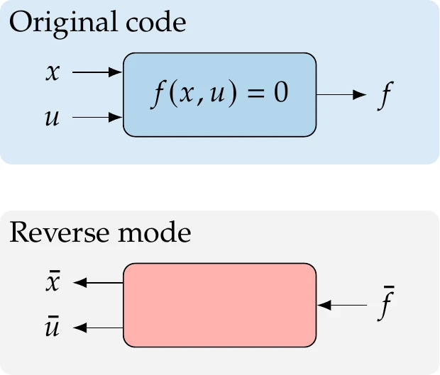
Figure 6.31:Applying reverse AD to the code that computes produces code that computes the partial derivatives of with respect to and .
Recall that we must first run the entire original code that computes and . Then we can run the AD code with the desired seed. Suppose we want the derivative of the th component of . We would set and the other elements to zero. After running the AD code, we obtain and , which correspond to the rows of the respective matrix of partial terms, that is,
Thus, with each run of the AD code, we obtain the derivatives of one function with respect to all design variables and all state variables. One run is required for each element of . The reverse mode is advantageous if , .
The Jacobian can also be computed using AD. Because is typically sparse, the techniques covered in Section 6.8 significantly increase the efficiency of computing this matrix. This is a square matrix, so neither AD mode has an advantage over the other if we explicitly compute and store the whole matrix.
However, reverse-mode AD is advantageous when using an iterative method to solve the adjoint linear system (Equation 6.46). When using an iterative method, we do not form . Instead, we require products of the transpose of this matrix with some vector ,[19]
The elements of act as weights on the residuals and can be interpreted as a projection onto the direction of . Suppose we have the reverse AD code for the residual computation, as shown in Figure 6.32.
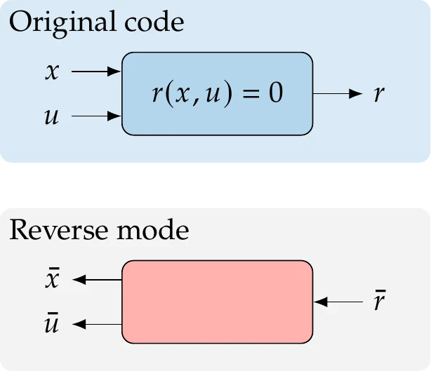
Figure 6.32:Applying reverse AD to the code that computes produces code that computes the partial derivatives of with respect to and .
This code requires a reverse seed , which determines the weights we want on each residual. Typically, a seed would have only one nonzero entry to find partial derivatives (e.g., setting would yield the first row of the Jacobian, ). However, to get the product in Equation 6.50, we require the seed to be weighted as . Then, we can compute the product by running the reverse AD code once to obtain .
The final term needed to compute total derivatives with the adjoint method is the last term in Equation 6.47, which can be written as
This is yet another transpose vector product that can be obtained using the same reverse AD code for the residuals, except that now the residual seed is , and the product we want is given by .
In sum, it is advantageous to use reverse-mode AD to compute the partial derivative terms for the adjoint equations, especially if the adjoint equations are solved using an iterative approach that requires only matrix-vector products. Similar techniques and arguments apply for the direct method, except that in that case, forward-mode AD is advantageous for computing the partial derivatives.
6.8 Sparse Jacobians and Graph Coloring
In this chapter, we have discussed various ways to compute a Jacobian of a model. If the Jacobian has many zero elements, it is said to be sparse. In many cases, we can take advantage of that sparsity to significantly reduce the computational time required to construct the Jacobian.
When applying a forward approach (forward-mode AD, finite differencing, or complex step), the cost of computing the Jacobian scales with . Each forward pass re-evaluates the model to compute one column of the Jacobian. For example, when using finite differencing, evaluations would be required. To compute the th column of the Jacobian, the input vector would be
We can significantly reduce the cost of computing the Jacobian depending on its sparsity pattern. As a simple example, consider a square diagonal Jacobian:
For this scenario, the Jacobian can be constructed with one evaluation rather than evaluations. This is because a given output depends on only one input . We could think of the outputs as independent functions. Thus, for finite differencing, rather than requiring input vectors with function evaluations, we can use one input vector, as follows:
allowing us to compute all the nonzero entries in one pass.[20]
Although the diagonal case is easy to understand, it is a special situation. To generalize this concept, let us consider the following matrix as an example:
A subset of columns that does not have more than one nonzero in any given row are said to be structurally orthogonal. In this example, the following sets of columns are structurally orthogonal: (1, 3), (1, 5), (2, 3), (2, 4, 5), (2, 6), and (4, 5). Structurally orthogonal columns can be combined, forming a smaller Jacobian that reduces the number of forward passes required. This reduced Jacobian is referred to as compressed. There is more than one way to compress this Jacobian, but in this case, the minimum number of compressed columns—referred to as colors—is three. In the following compressed Jacobian, we combine columns 1 and 3 (blue); columns 2, 4, and 5 (red); and leave column 6 on its own (black):
For finite differencing, complex step, and forward-mode AD, only compression among columns is possible. Reverse mode AD allows compression among the rows. The concept is the same, but instead, we look for structurally orthogonal rows. One such compression is as follows:
AD can also be used even more flexibly when both modes are used: forward passes to evaluate groups of structurally orthogonal columns and reverse passes to evaluate groups of structurally orthogonal rows. Rather than taking incremental steps in each direction as is done in finite differencing, we set the AD seed vector with 1s in the directions we wish to evaluate, similar to how the seed is set for directional derivatives, as discussed in Section 6.6.
For these small Jacobians, it is straightforward to determine how to compress the matrix in the best possible way. For a large matrix, this is not so easy. One approach is to use graph coloring. This approach starts by building a graph where the vertices represent the row and column indices, and the edges represent nonzero entries in the Jacobian. Then, algorithms are applied to this graph that estimate the fewest number of “colors” (orthogonal columns) using heuristics. Graph coloring is a large field of research, where derivative computation is one of many applications.[21]
6.9 Unified Derivatives Equation
Now that we have introduced all the methods for computing derivatives, we will see how they are connected. For example, we have mentioned that the direct and adjoint methods are analogous to the forward and reverse mode of AD, respectively, but we did not show this mathematically. The unified derivatives equation (UDE) expresses both methods.25 Also, the implicit analytic methods from Section 6.7 assumed one set of implicit equations () and one set of explicit functions (). The UDE formulates the derivative computation for systems with mixed sets of implicit and explicit equations.
We first derive the UDE from basic principles and give an intuitive explanation of the derivative terms. Then, we show how we can use the UDE to handle implicit and explicit equations. We also show how the UDE can retrieve the direct and adjoint equations. Finally, we show how the UDE is connected to AD.
6.9.1 UDE Derivation
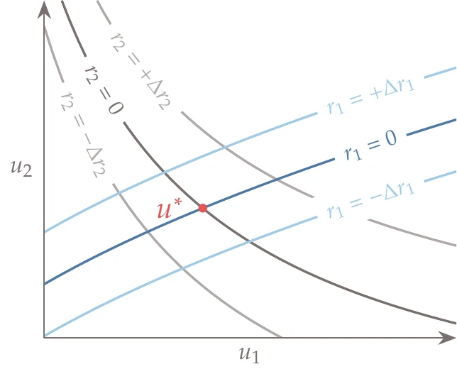
Figure 6.35:Solution of a system of two equations expressed by residuals.
Suppose we have a set of residual equations with the same number of unknowns,
and that there is at least one solution such that . Such a solution can be visualized for , as shown in Figure 6.35.
These residuals are general: each one can depend on any subset of the variables and can be truly implicit functions or explicit functions converted to the implicit form (see Section 3.3 and Example 3.3). The total differentials for these residuals are
These represent first-order changes in due to perturbations in . The differentials of can be visualized as perturbations in the space of the variables. The differentials of can be visualized as linear changes to the surface defined by , as illustrated in Figure 6.36.
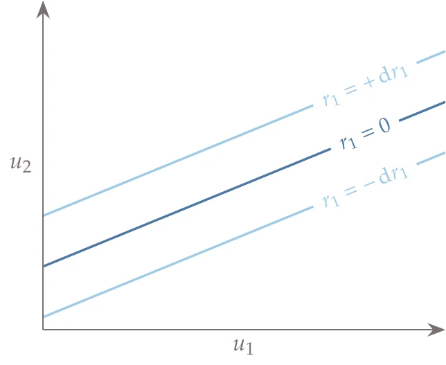
Figure 6.36:The differential can be visualized as a linearized (first-order) change of the contour value.
We can write the differentials (Equation 6.61) in matrix form as
The partial derivatives in the matrix are derivatives of the expressions for with respect to that can be obtained symbolically, and they are in general functions of . The vector of differentials represents perturbations in that can be solved for a given vector of changes .
Now suppose that we are at a solution , such that . All the partial derivatives () can be evaluated at . When all entries in are zero, then the solution of this linear system yields . This is because if there is no disruption in the residuals that are already zero, the variables do not need to change either.
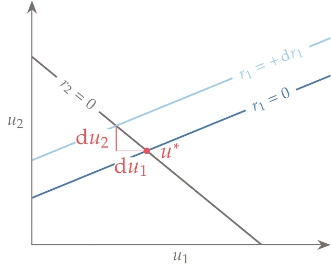
Figure 6.37:The total derivatives and represent the first-order changes needed to satisfy a perturbation while keeping .
How is this linear system useful? With these differentials, we can choose different combinations of to obtain any total derivatives that we want. For example, we can get the total derivatives of with respect to a single residual by keeping while setting all the other differentials to zero (). The visual interpretation of this total derivative is shown in Figure 6.37 for and . Setting in Equation 6.62 and moving to the denominator, we obtain the following linear system:[22]
Doing the same for all , we get the following linear systems:
Solving these linear systems yields the total derivatives of all the elements of with respect to all the elements of . We can write this more compactly in matrix form as
This is the forward form of the UDE.
The total derivatives might not seem like the derivatives in which we are interested. Based on the implicit analytic methods derived in Section 6.7.2, these look like derivatives of states with respect to residuals, not the derivatives that we ultimately want to compute (). However, we will soon see that with the appropriate choice of and , we can obtain a linear system that solves for the total derivatives we want.
With Equation 6.65, we can solve one column at a time. Similar to AD, we can also solve for the rows instead by transposing the systems as [23]
which is the reverse form of the UDE.
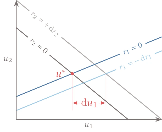
Figure 6.38:The total derivatives and represent the first-order change in resulting from perturbations and .
Now, each column yields —the total derivative of one variable with respect to all the residuals. This total derivative is interpreted visually in Figure 6.38.
The usefulness of the total derivative Jacobian might still not be apparent. In the next section, we explain how to set up the UDE to include in the UDE unknowns ().
6.9.2 UDE for Mixed Implicit and Explicit Components
In the previous section, the UDE was derived based on residual equations. The equations were written in implicit form, but there was no assumption on whether the equations were implicit or explicit. Because we can write an explicit equation in implicit form (see Section 3.3 and Example 3.3), the UDE allows a mix of implicit and explicit set of equations, which we now call components.
To derive the implicit analytic equations in Section 6.7, we considered two components: an implicit component that determines by solving and an explicit component that computes the functions of interest, .
We can recover the implicit analytic differentiation equations (direct and adjoint) from the UDE by defining a set of variables that concatenates the state variables with inputs and outputs as follows:
This is a vector with variables. For the residuals, we need a vector with the same size. We can obtain this by realizing that the residuals associated with the inputs and outputs are just explicit functions that can be written in implicit form. Then, we have
Here, we distinguish (the actual variable in the UDE system) from (a given input) and (the variable) from (an explicit function of and ). Similarly, is the vector of variables associated with the residual and is the residual function itself.
Taking the differential of the residuals, and considering only one of them to be nonzero at a time, we obtain,
Using these variable and residual definitions in Equation 6.65 and Equation 6.66 yields the full UDE shown in Figure 6.40, where the block we ultimately want to compute is .
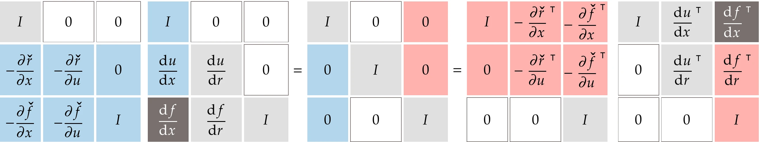
Figure 6.40:The direct and adjoint methods can be recovered from the UDE.
To compute using the forward UDE (left-hand side of the equation in Figure 6.40, we can ignore all but three blocks in the total derivatives matrix: , , and . By multiplying these blocks and using the definition , we recover the direct linear system (Equation 6.43) and the total derivative equation (Equation 6.44).
To compute using the reverse UDE (right-hand side of the equation in Figure 6.40), we can ignore all but three blocks in the total derivatives matrix: , , and . By multiplying these blocks and defining , we recover the adjoint linear system (Equation 6.46) and the corresponding total derivative equation (Equation 6.47).
The definition of here is significant because, as mentioned in Section 6.7.2, the adjoint vector is the total derivative of the objective function with respect to the governing equation residuals.
By defining one implicit component (associated with ) and two explicit components (associated with and ), we have retrieved the direct and adjoint methods from the UDE. In general, we can define an arbitrary number of components, so the UDE provides a mathematical framework for computing the derivatives of coupled systems. Furthermore, each component can be implicit or explicit, so the UDE can handle an arbitrary mix of components. All we need to do is to include the desired states in the UDE augmented variables vector (Equation 6.69) and the corresponding residuals in the UDE residuals vector (Equation 6.70). We address coupled systems in Section 13.3.3 and use the UDE in Section 13.2.6, where we extend it to coupled systems with a hierarchy of components.
6.9.3 Recovering AD
Now we will see how we can recover AD from the UDE. First, we define the UDE variables associated with each operation or line of code (assuming all loops have been unrolled), such that and
Recall from Section 6.6.1 that each variable is an explicit function of the previous ones.
To define the appropriate residuals, we use the same technique from before to convert an explicit function into implicit form by moving all the terms in the left-hand side to obtain
The distinction between and is that represents variables that are considered independent in the UDE, whereas represents the explicit expressions. Of course, the values for these become equal once the system is solved. Similar to the differentials in Equation 6.71,
Taking the partial derivatives of the residuals (Equation 6.73) with respect to (Equation 6.72), and replacing the total derivatives in the forward form of the UDE (Equation 6.65) with the new symbols yields
This equation is the matrix form of the AD forward chain rule (Equation 6.21), where each column of the total derivative matrix corresponds to the tangent vector () for the chosen input variable. As observed in Figure 6.16, the partial derivatives form a lower triangular matrix. The Jacobian we ultimately want to compute () is composed of a subset of derivatives in the bottom-left corner near the term. To compute these derivatives, we need to perform forward substitution and compute one column of the total derivative matrix at a time, where each column is associated with the inputs of interest.
Similarly, the reverse form of the UDE (Equation 6.66) yields the transpose of Equation 6.74,
This is equivalent to the AD reverse chain rule (Equation 6.26), where each column of the total derivative matrix corresponds to the gradient vector () for the chosen output variable. The partial derivatives now form an upper triangular matrix, as previously shown in Figure 6.21. The derivatives of interest are now near the top-right corner of the total derivative matrix near the term. To compute these derivatives, we need to perform back substitutions, computing one column of the matrix at a time.
6.10 Summary
Derivatives are useful in many applications beyond optimization. This chapter introduced the methods available to compute the first derivatives of the outputs of a model with respect to its inputs. In optimization, the outputs are usually the objective function and the constraint functions, and the inputs are the design variables. The typical characteristics of the available methods are compared in Table 4.
Table 4:Characteristics of the various derivative computation methods. Some of these characteristics are problem or implementation dependent, so these are not universal.
| Accuracy | Scalability | Ease of | Implicit | |
| implementation | functions | |||
| Symbolic | Hard | |||
| Finite difference | Easy | |||
| Complex step | Intermediate | |||
| AD | Intermediate | |||
| Implicit analytic | Hard |
Symbolic differentiation is accurate but only scalable for simple, explicit functions of low dimensionality. Therefore, it is necessary to compute derivatives numerically. Although it is generally intractable or inefficient for many engineering models, symbolic differentiation is used by AD at each line of code and in implicit analytic methods to derive expressions for computing the required partial derivatives.
Finite-difference approximations are popular because they are easy to implement and can be applied to any model, including black-box models. The downsides are that these approximations are not accurate, and the cost scales linearly with the number of variables. Many of the issues practitioners experience with gradient-based optimization can be traced to errors in the gradients when algorithms automatically compute these gradients using finite differences.
The complex-step method is accurate and relatively easy to implement. It usually requires some changes to the analysis source code, but this process can be scripted. The main advantage of the complex-step method is that it produces analytically accurate derivatives. However, like the finite-difference method, the cost scales linearly with the number of inputs, and each simulation requires more effort because of the complex arithmetic.
AD produces analytically accurate derivatives, and many implementations can be fully automated. The implementation requires access to the source code but is still relatively straightforward to apply. The computational cost of forward-mode AD scales with the number of inputs, and the reverse mode scales with the number of outputs. The scaling factor for the forward mode is generally lower than that for finite differences. The cost of reverse-mode AD is independent of the number of design variables.
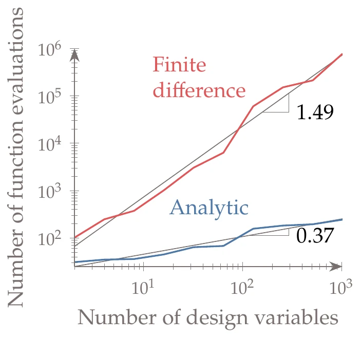
Figure 6.43:Efficient gradient computation with an analytic method improves the scalability of gradient-based algorithms compared to finite differencing. In this case, we show the results for the -dimensional Rosenbrock, where the cost of computing the derivatives analytically is independent of .
Implicit analytic methods (direct and adjoint) are accurate and scalable but require significant implementation effort. These methods are exact (depending on how the partial derivatives are obtained), and like AD, they provide both forward and reverse modes with the same scaling advantages. Gradient-based optimization using the adjoint method is a powerful combination that scales well with the number of variables, as shown in Figure 6.43. The disadvantage is that because implicit methods are intrusive, they require considerable development effort.
A hybrid approach where the partial derivatives for the implicit analytic equations are computed with AD is generally recommended. This hybrid approach is computationally more efficient than AD while reducing the implementation effort of implicit analytic methods and ensuring accuracy.
The UDE encapsulates all the derivative computation methods in a single linear system. Using the UDE, we can formulate the derivative computation for an arbitrary system of mixed explicit and implicit components. This will be used in Section 13.2.6 to develop a mathematical framework for solving coupled systems and computing the corresponding derivatives.
Problems
Here, is the difference between the eccentric and mean anomalies, is the mean anomaly, and the eccentricity is set to 1. For more details, see Exercise 6 and .
This method originated with the work of 1 who developed formulas that use complex arithmetic for computing the derivatives of real functions of arbitrary order with arbitrary order truncation error, much like the Taylor series combination approach in finite differences. Later, 2 observed that the simplest of these formulas was convenient for computing first derivatives.
For more details on the problematic functions and how to implement the complex-step method in various programming languages, see 3 A summary, implementation guide, and scripts are available at: http://
bit .ly /complexstep A stack, also known as last in, first out (LIFO), is a data structure that stores a one-dimensional array. We can only add an element to the top of the stack (push) and take the element from the top of the stack (pop).
The overloading of ‘’” computes and then the overloading of “” computes .
This chain rule can be derived by writing the total differential of as
and then “dividing” it by . See Section A.2 for more background on differentials.
The adjoint vector can also be interpreted as a Lagrange multiplier vector associated with equality constraints . Defining the Lagrangian and differentiating it with respect to , we get
Thus, the total derivatives are the derivatives of this Lagrangian.
The displacements do change with the areas but only through the solution of the governing equations, which are not considered when taking partial derivatives.
This is not true for large displacements, but we assume small displacements .
Although ultimately, the areas do change the stresses, they do so only through changes in the displacements.
Usually, the stiffness matrix is symmetric, and . This means that the solver for displacements can be repurposed for adjoint computation by setting the right-hand side shown here instead of the loads. For that reason, this right-hand side is sometimes called a pseudo-load.
See Iterative Methods for more details on iterative solvers.
As explained in Section A.2, we take the liberty of treating differentials algebraically and skip a more rigorous and lengthy proof.
Normally, for two matrices and , , but in this case,
.
- Lyness, J. N., & Moler, C. B. (1967). Numerical differentiation of analytic functions. SIAM Journal on Numerical Analysis, 4(2), 202–210. 10.1137/0704019
- Squire, W., & Trapp, G. (1998). Using complex variables to estimate derivatives of real functions. SIAM Review, 40(1), 110–112. 10.1137/S003614459631241X
- Martins, J. R. R. A., Sturdza, P., & Alonso, J. J. (2003). The complex-step derivative approximation. ACM Transactions on Mathematical Software, 29(3), 245–262. 10.1145/838250.838251
- Lantoine, G., Russell, R. P., & Dargent, T. (2012). Using multicomplex variables for automatic computation of high-order derivatives. ACM Transactions on Mathematical Software, 38(3), 1–21. 10.1145/2168773.2168774
- Fike, J. A., & Alonso, J. J. (2012). Automatic differentiation through the use of hyper-dual numbers for second derivatives. In S. Forth, P. Hovland, E. Phipps, J. Utke, & A. Walther (Eds.), Recent Advances in Algorithmic Differentiation (pp. 163–173). Springer. 10.1007/978-3-642-30023-3_15
- Griewank, A. (2000). Evaluating Derivatives. SIAM. 10.1137/1.9780898717761
- Naumann, U. (2011). The Art of Differentiating Computer Programs—An Introduction to Algorithmic Differentiation. SIAM. https://books.google.ca/books/about/The_Art_of_Differentiating_Computer_Prog.html?id=OgQuUR4nLu0C
- Utke, J., Naumann, U., Fagan, M., Tallent, N., Strout, M., Heimbach, P., Hill, C., & Wunsch, C. (2008). OpenAD/F: A modular open-source tool for automatic differentiation of Fortran codes. ACM Transactions on Mathematical Software, 34(4). 10.1145/1377596.1377598
- Hascoet, L., & Pascual, V. (2013). The Tapenade automatic differentiation tool: Principles, model, and specification. ACM Transactions on Mathematical Software, 39(3), 20:1-20:43. 10.1145/2450153.2450158
- Griewank, A., Juedes, D., & Utke, J. (1996). Algorithm 755: ADOL-C: A package for the automatic differentiation of algorithms written in C\slash C++. ACM Transactions on Mathematical Software, 22(2), 131–167. 10.1145/229473.229474
- Wiltschko, A. B., van Merriënboer, B., & Moldovan, D. (2017). Tangent: automatic differentiation using source code transformation in Python. https://arxiv.org/abs/1711.02712
- Bradbury, J., Frostig, R., Hawkins, P., Johnson, M. J., Leary, C., Maclaurin, D., Necula, G., Paszke, A., VanderPlas, J., Wanderman-Milne, S., & Zhang, Q. (2018). JAX: Composable Transformations of Python+NumPy Programs (0.2.5). http://github.com/google/jax
- Revels, J., Lubin, M., & Papamarkou, T. (2016). Forward-mode automatic differentiation in Julia. In ArXiv e-prints. https://arxiv.org/abs/1607.07892
- Neidinger, R. D. (2010). Introduction to automatic differentiation and MATLAB object-oriented programming. SIAM Review, 52(3), 545–563. 10.1137/080743627
- Betancourt, M. (2018). A geometric theory of higher-order automatic differentiation. https://arxiv.org/abs/1812.11592