7 Gradient-Free Optimization
Gradient-free algorithms fill an essential role in optimization. The gradient-based algorithms introduced in Chapter 4 are efficient in finding local minima for high-dimensional nonlinear problems defined by continuous smooth functions. However, the assumptions made for these algorithms are not always valid, which can render these algorithms ineffective. Also, gradients might not be available when a function is given as a black box.
In this chapter, we introduce only a few popular representative gradient-free algorithms. Most are designed to handle unconstrained functions only, but they can be adapted to solve constrained problems by using the penalty or filtering methods introduced in Chapter 5. We start by discussing the problem characteristics relevant to the choice between gradient-free and gradient-based algorithms and then give an overview of the types of gradient-free algorithms.
7.1 When to Use Gradient-Free Algorithms
Gradient-free algorithms can be useful when gradients are not available, such as when dealing with black-box functions. Although gradients can always be approximated with finite differences, these approximations suffer from potentially significant inaccuracies (see Section 6.4.2). Gradient-based algorithms require a more experienced user because they take more effort to set up and run. Overall, gradient-free algorithms are easier to get up and running but are much less efficient, particularly as the dimension of the problem increases.
One significant advantage of gradient-free algorithms is that they do not assume function continuity. For gradient-based algorithms, function smoothness is essential when deriving the optimality conditions, both for unconstrained functions and constrained functions. More specifically, the Karush–Kuhn–Tucker (KKT) conditions (Equation 5.11) require that the function be continuous in value (), gradient (), and Hessian () in at least a small neighborhood of the optimum.
If, for example, the gradient is discontinuous at the optimum, it is undefined, and the KKT conditions are not valid. Away from optimum points, this requirement is not as stringent. Although gradient-based algorithms work on the same continuity assumptions, they can usually tolerate the occasional discontinuity, as long as it is away from an optimum point. However, for functions with excessive numerical noise and discontinuities, gradient-free algorithms might be the only option.
Many considerations are involved when choosing between a gradient-based and a gradient-free algorithm. Some of these considerations are common sources of misconception. One problem characteristic often cited as a reason for choosing gradient-free methods is multimodality. Design space multimodality can be a result of an objective function with multiple local minima. In the case of a constrained problem, the multimodality can arise from the constraints that define disconnected or nonconvex feasible regions.
As we will see shortly, some gradient-free methods feature a global search that increases the likelihood of finding the global minimum. This feature makes gradient-free methods a common choice for multimodal problems. However, not all gradient-free methods are global search methods; some perform only a local search. Additionally, even though gradient-based methods are by themselves local search methods, they are often combined with global search strategies, as discussed in Tip 4.8. It is not necessarily true that a global search, gradient-free method is more likely to find a global optimum than a multistart gradient-based method. As always, problem-specific testing is needed.
Furthermore, it is assumed far too often that any complex problem is multimodal, but that is frequently not the case. Although it might be impossible to prove that a function is unimodal, it is easy to prove that a function is multimodal simply by finding another local minimum. Therefore, we should not make any assumptions about the multimodality of a function until we show definite multiple local minima. Additionally, we must ensure that perceived local minima are not artificial minima arising from numerical noise.
Another reason often cited for using a gradient-free method is multiple objectives. Some gradient-free algorithms, such as the genetic algorithm discussed in this chapter, can be naturally applied to multiple objectives. However, it is a misconception that gradient-free methods are always preferable just because there are multiple objectives. This topic is introduced in Chapter 9.
Another common reason for using gradient-free methods is when there are discrete design variables. Because the notion of a derivative with respect to a discrete variable is invalid, gradient-based algorithms cannot be used directly (although there are ways around this limitation, as discussed in Chapter 8). Some gradient-free algorithms can handle discrete variables directly.
The preceding discussion highlights that although multimodality, multiple objectives, or discrete variables are commonly mentioned as reasons for choosing a gradient-free algorithm, these are not necessarily automatic decisions, and careful consideration is needed. Assuming a choice exists (i.e., the function is not too noisy), one of the most relevant factors when choosing between a gradient-free and a gradient-based approach is the dimension of the problem.
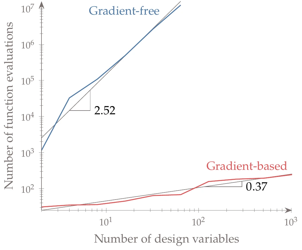
Figure 7.1:Cost of optimization for increasing number of design variables in the -dimensional Rosenbrock function. A gradient-free algorithm is compared with a gradient-based algorithm, with gradients computed analytically. The gradient-based algorithm has much better scalability.
Figure 7.1 shows how many function evaluations are required to minimize the -dimensional Rosenbrock function for varying numbers of design variables. Two classes of algorithms are shown in the plot: gradient-free and gradient-based algorithms. The gradient-based algorithm uses analytic gradients in this case. Although the exact numbers are problem dependent, similar scaling has been observed in large-scale computational fluid dynamics–based optimization.1 The general takeaway is that for small-size problems (usually variables2), gradient-free methods can be useful in finding a solution. Furthermore, because gradient-free methods usually take much less developer time to use, a gradient-free solution may even be preferable for these smaller problems. However, if the problem is large in dimension, then a gradient-based method may be the only viable method despite the need for more developer time.
7.2 Classification of Gradient-Free Algorithms
There is a much wider variety of gradient-free algorithms compared with their gradient-based counterparts. Although gradient-based algorithms tend to perform local searches, have a mathematical rationale, and be deterministic, gradient-free algorithms exhibit different combinations of these characteristics. We list some of the most widely known gradient-free algorithms in Table 1 and classify them according to the characteristics introduced in Figure 1.22.[1]
Table 1:Classification of gradient-free optimization methods using the characteristics of Figure 1.22.
| Search | Algorithm | Function evaluation | Stochas- ticity | |||||
| Local | Global | Mathematical | Heuristic | Direct | Surrogate | Deterministic | Stochastic | |
| Nelder–Mead | ||||||||
| GPS | ||||||||
| MADS | ||||||||
| Trust region | ||||||||
| Implicit filtering | ||||||||
| DIRECT | ||||||||
| MCS | ||||||||
| EGO | ||||||||
| Hit and run | ||||||||
| Evolutionary | ||||||||
Local search, gradient-free algorithms that use direct function evaluations include the Nelder–Mead algorithm, generalized pattern search (GPS), and mesh-adaptive direct search (MADS). Although classified as local search in the table, the latter two methods are frequently used with globalization approaches. The Nelder–Mead algorithm (which we detail in Section 7.3) is heuristic, whereas the other two are not.
GPS and MADS (discussed in Section 7.4) are examples of derivative-free optimization (DFO) algorithms, which, despite the name, do not include all gradient-free algorithms. DFO algorithms are understood to be largely heuristic-free and focus on local search.[2] GPS is a family of methods that iteratively seek an improvement using a set of points around the current point. In its simplest versions, GPS uses a pattern of points based on the coordinate directions, but more sophisticated versions use a more general set of vectors. MADS improves GPS algorithms by allowing a much larger set of such vectors and improving convergence.
Model-based, local search algorithms include trust-region algorithms and implicit filtering. The model is an analytic approximation of the original function (also called a surrogate model), and it should be smooth, easy to evaluate, and accurate in the neighborhood of the current point. The trust-region approach detailed in Section 4.5 can be considered gradient-free if the surrogate model is constructed using just evaluations of the original function without evaluating its gradients. This does not prevent the trust-region algorithm from using gradients of the surrogate model, which can be computed analytically. Implicit filtering methods extend the trust-region method by adding a surrogate model of the function gradient to guide the search. This effectively becomes a gradient-based method applied to the surrogate model instead of evaluating the function directly, as done for the methods in Chapter 4.
Global search algorithms can be broadly classified as deterministic or stochastic, depending on whether they include random parameter generation within the optimization algorithm.
Deterministic, global search algorithms can be either direct or model based. Direct algorithms include Lipschitzian-based partitioning techniques—such as the “divide a hyperrectangle” (DIRECT) algorithm detailed in Section 7.5 and branch-and-bound search (discussed in Chapter 8)—and multilevel coordinate search (MCS).
The DIRECT algorithm selectively divides the space of the design variables into smaller and smaller -dimensional boxes—hyperrectangles. It uses mathematical arguments to decide which boxes should be subdivided. Branch-and-bound search also partitions the design space, but it estimates lower and upper bounds for the optimum by using the function variation between partitions. MCS is another algorithm that partitions the design space into boxes, where a limit is imposed on how small the boxes can get based on the number of times it has been divided.
Global-search algorithms based on surrogate models are similar to their local search counterparts. However, they use surrogate models to reproduce the features of a multimodal function instead of convex surrogate models. One of the most widely used of these algorithms is efficient global optimization (EGO), which employs kriging surrogate models and uses the idea of expected improvement to maximize the likelihood of finding the optimum more efficiently (surrogate modeling techniques, including kriging are introduced in Chapter 10, which also described EGO). Other algorithms use radial basis functions (RBFs) as the surrogate model and also maximize the probability of improvement at new iterates.
Stochastic algorithms rely on one or more nondeterministic procedures; they include hit-and-run algorithms and the broad class of evolutionary algorithms. When performing benchmarks of a stochastic algorithm, you should run a large enough number of optimizations to obtain statistically significant results.
Hit-and-run algorithms generate random steps about the current iterate in search of better points. A new point is accepted when it is better than the current one, and this process repeats until the point cannot be improved.
What constitutes an evolutionary algorithm is not well defined.[3] Evolutionary algorithms are inspired by processes that occur in nature or society. There is a plethora of evolutionary algorithms in the literature, thanks to the fertile imagination of the research community and a never-ending supply of phenomena for inspiration.[4]These algorithms are more of an analogy of the phenomenon than an actual model. They are, at best, simplified models and, at worst, barely connected to the phenomenon. Nature-inspired algorithms tend to invent a specific terminology for the mathematical terms in the optimization problem. For example, a design point might be called a “member of the population”, or the objective function might be the “fitness”.
The vast majority of evolutionary algorithms are population based, which means they involve a set of points at each iteration instead of a single one (we discuss a genetic algorithm in Section 7.6 and a particle swarm method in Section 7.7). Because the population is spread out in the design space, evolutionary algorithms perform a global search. The stochastic elements in these algorithms contribute to global exploration and reduce the susceptibility to getting stuck in local minima. These features increase the likelihood of getting close to the global minimum but by no means guarantee it. The algorithm may only get close because heuristic algorithms have a poor convergence rate, especially in higher dimensions, and because they lack a first-order mathematical optimality criterion.
This chapter covers five gradient-free algorithms: the Nelder–Mead algorithm, GPS, the DIRECT method, genetic algorithms, and particle swarm optimization. A few other algorithms that can be used for continuous gradient-free problems (e.g., simulated annealing and branch and bound) are covered in Chapter 8 because they are more frequently used to solve discrete problems. In Chapter 10, on surrogate modeling, we discuss kriging and efficient global optimization.
7.3 Nelder–Mead Algorithm
The simplex method of Nelder & Mead (1965) is a deterministic, direct-search method that is among the most cited gradient-free methods. It is also known as the nonlinear simplex—not to be confused with the simplex algorithm used for linear programming, with which it has nothing in common. To avoid ambiguity, we will refer to it as the Nelder–Mead algorithm.
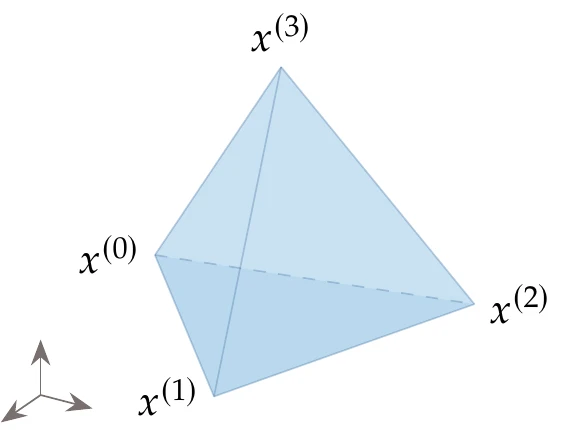
Figure 7.2:A simplex for has four vertices.
The Nelder–Mead algorithm is based on a simplex, which is a geometric figure defined by a set of points in the design space of variables, . Each point represents a design (i.e., a full set of design variables). In two dimensions, the simplex is a triangle, and in three dimensions, it becomes a tetrahedron (see Figure 7.2).
Each optimization iteration corresponds to a different simplex. The algorithm modifies the simplex at each iteration using five simple operations. The sequence of operations to be performed is chosen based on the relative values of the objective function at each of the points.
The first step of the simplex algorithm is to generate points based on an initial guess for the design variables. This could be done by simply adding steps to each component of the initial point to generate new points. However, this will generate a simplex with different edge lengths, and equal-length edges are preferable. Suppose we want the length of all sides to be and that the first guess is . The remaining points of the simplex, , can be computed by
where is a vector whose components are defined by
Figure 7.3 shows a starting simplex for a two-dimensional problem.
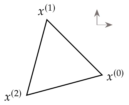
Figure 7.3:Starting simplex for .
At any given iteration, the objective is evaluated for every point, and the points are ordered based on the respective values of , from the lowest to the highest. Thus, in the ordered list of simplex points , the best point is , and the worst one is .
The Nelder–Mead algorithm performs five main operations on the simplex to create a new one: reflection, expansion, outside contraction, inside contraction, and shrinking, as shown in Figure 7.4. Except for shrinking, each of these operations generates a new point,
where is a scalar, and is the centroid of all the points except for the worst one, that is,
This generates a new point along the line that connects the worst point, , and the centroid of the remaining points, . This direction can be seen as a possible descent direction.
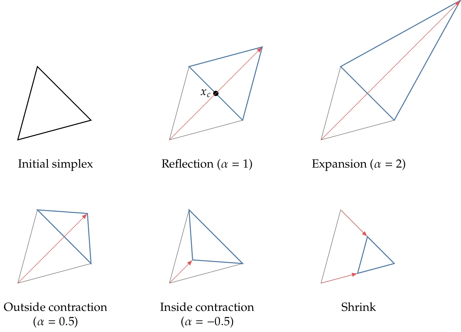
Figure 7.4:Nelder–Mead algorithm operations for .
Each iteration aims to replace the worst point with a better one to form a new simplex. Each iteration always starts with reflection, which generates a new point using Equation 7.3 with , as shown in Figure 7.4. If the reflected point is better than the best point, then the “search direction” was a good one, and we go further by performing an expansion using Equation 7.3 with . If the reflected point is between the second-worst and the worst point, then the direction was not great, but it improved somewhat. In this case, we perform an outside contraction (). If the reflected point is worse than our worst point, we try an inside contraction instead (). Shrinking is a last-resort operation that we can perform when nothing along the line connecting and produces a better point. This operation consists of reducing the size of the simplex by moving all the points closer to the best point,
where .
Algorithm 7.1 details how a new simplex is obtained for each iteration. In each iteration, the focus is on replacing the worst point with a better one instead of improving the best. The corresponding flowchart is shown in Figure 7.5.
The cost for each iteration is one function evaluation if the reflection is accepted, two function evaluations if an expansion or contraction is performed, and evaluations if the iteration results in shrinking. Although we could parallelize the evaluations when shrinking, it would not be worthwhile because the other operations are sequential.
There several ways to quantify the convergence of the simplex method. One straightforward way is to use the size of simplex, that is,
and specify that it must be less than a certain tolerance. Another measure of convergence we can use is the standard deviation of the function value,
where is the mean of the function values. Another possible convergence criterion is the difference between the best and worst value in the simplex. Nelder–Mead is known for occasionally converging to non-stationary points, so you should check the result if possible.
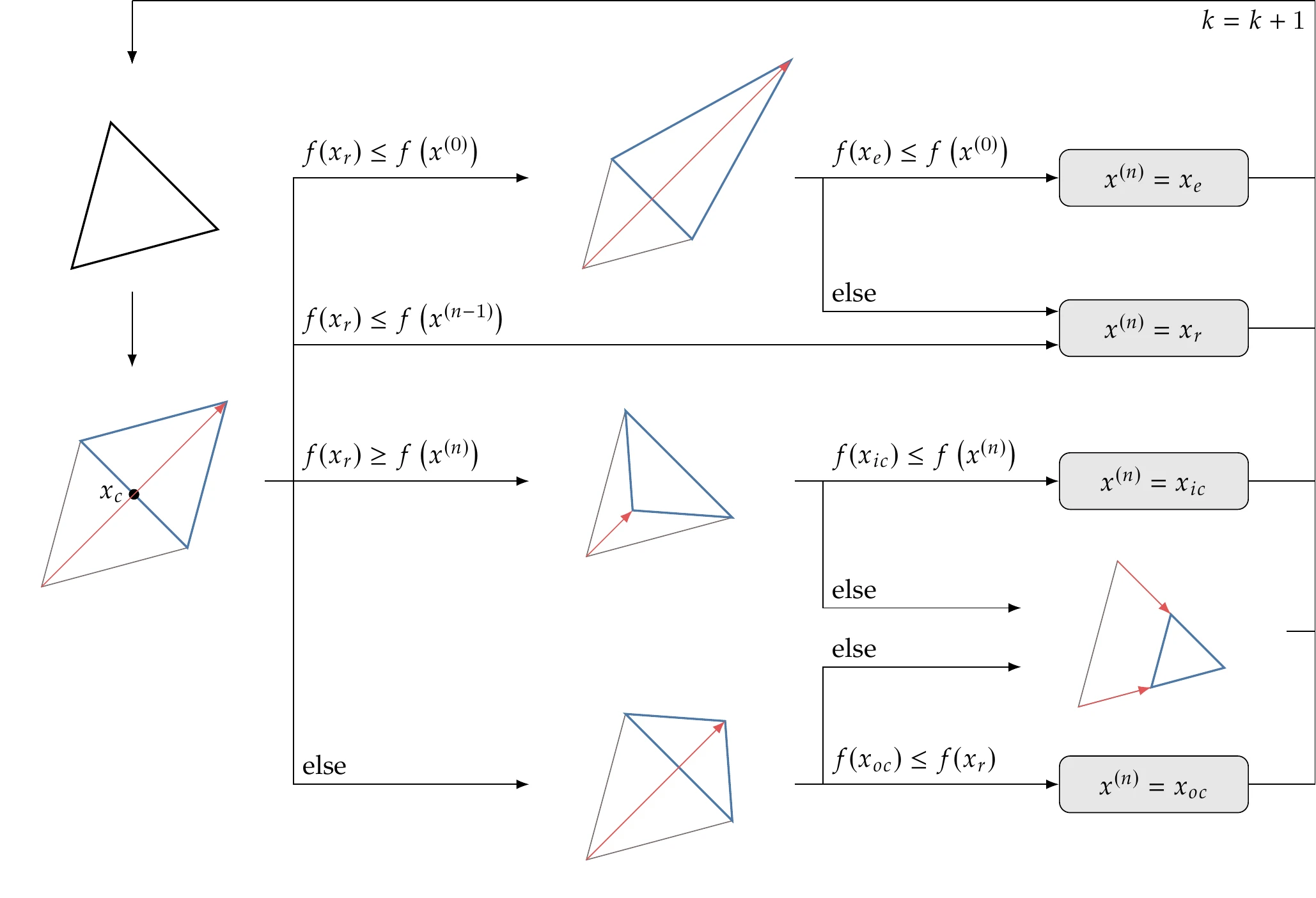
Figure 7.5:Flowchart of Nelder–Mead (Algorithm 7.1).
Like most direct-search methods, Nelder–Mead cannot directly handle constraints. One approach to handling constraints would be to use a penalty method (discussed in Section 5.4) to form an unconstrained problem. In this case, the penalty does not need not be differentiable, so a linear penalty method would suffice.
7.4 Generalized Pattern Search
GPS builds upon the ideas of a coordinate search algorithm. In coordinate search, we evaluate points along a mesh aligned with the coordinate directions, move toward better points, and shrink the mesh when we find no improvement nearby. Consider a two-dimensional coordinate search for an unconstrained problem. At a given point , we evaluate points that are a distance away in all coordinate directions, as shown in Figure 7.7. If the objective function improves at any of these points (four points in this case), we recenter with at the most improved point, keep the mesh size the same at , and start with the next iteration. Alternatively, if none of the points offers an improvement, we keep the same center () and shrink the mesh to . This process repeats until it meets some convergence criteria.
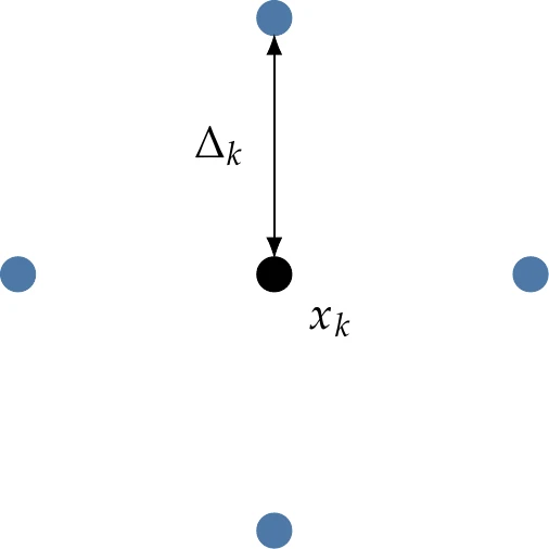
Figure 7.7:Local mesh for a two-dimensional coordinate search at iteration .
We now explore various ways in which GPS improves coordinate search. Coordinate search moves along coordinate directions, but this is not necessarily desirable. Instead, the GPS search directions only need to form a positive spanning set. Given a set of directions , the set is a positive spanning set if the vectors are linearly independent and a nonnegative linear combination of these vectors spans the -dimensional space.[5]Coordinate vectors fulfill this requirement, but there is an infinite number of options. The vectors are referred to as positive spanning directions. We only consider linear combinations with positive multipliers, so in two dimensions, the unit coordinate vectors and are not sufficient to span two-dimensional space; however, and are sufficient.
For a given dimension , the largest number of vectors that could be used while remaining linearly independent (known as the maximal set) is . Conversely, the minimum number of possible vectors needed to span the space (known as the minimal set) is . These sizes are necessary but not sufficient conditions.
Some algorithms randomly generate a positive spanning set, whereas other algorithms require the user to specify a set based on knowledge of the problem. The positive spanning set need not be fixed throughout the optimization. A common default for a maximal set is the set of coordinate directions . In three dimensions, this would be:
A potential default minimal set is the positive coordinate directions and a vector filled with -1 (or more generally, the negative sum of the other vectors). As an example in three dimensions:
Figure 7.8 shows an example maximal set (four vectors) and minimal set (three vectors) for a two-dimensional problem.
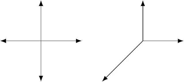
Figure 7.8:A maximal set of positive spanning vectors in two dimensions (left) and a minimal set (right).
These direction vectors are then used to create a mesh. Given a current center point , which is the best point found so far, and a mesh size , the mesh is created as follows:
For example, in two dimensions, if the current point is , the mesh size is , and we use the coordinate directions for , then the mesh points would be .
The evaluation of points in the mesh is called polling or a poll. In the coordinate search example, we evaluated every point in the mesh, which is usually inefficient. More typically, we use opportunistic polling, which terminates polling at the first point that offers an improvement. Figure 7.9 shows a two-dimensional example where the order of evaluation is . Because we found an improvement at , we do not continue evaluating and .
![A two-dimensional example of opportunistic polling with d_1 = [1, 0], d_2 = [0, 1] , d_3 = [-1, 0], d_4 = [0, -1]. An improvement in f was found at d_2, so we do not evaluate d_3 and d_4 (shown with a faded color).](https://mdobook.github.io/html/build/gps3-32853c27c5abc6f0cb0b60240c1738a7.webp)
Figure 7.9:A two-dimensional example of opportunistic polling with . An improvement in was found at , so we do not evaluate and (shown with a faded color).
Opportunistic polling may not yield the best point in the mesh, but the improvement in efficiency is usually worth the trade-off. Some algorithms add a user option for utilizing a full poll, in which case all points in the mesh are evaluated. If more than one point offers a reduction, the best one is accepted. Another approach that is sometimes used is called dynamic polling. In this approach, a successful poll reorders the direction vectors so that the direction that was successful last time is checked first in the next poll.
GPS consists of two phases: a search phase and a poll phase. The search phase is global, whereas the poll phase is local. The search phase is intended to be flexible and is not specified by the GPS algorithm. Common options for the search phase include the following:
No search phase.
A mesh search, similar to polling but with large spacing across the domain.
An alternative solver, such as Nelder–Mead or a genetic algorithm.
A surrogate model, which could then use any number of solvers that include gradient-based methods. This approach is often used when the function is expensive, and a lower-fidelity surrogate can guide the optimizer to promising regions of the larger design space.
Random evaluation using a space-filling method (see Section 10.2).
The type of search can change throughout the optimization. Like the polling phase, the goal of the search phase is to find a better point (i.e., ) but within a broader domain. We begin with a search at every iteration. If the search fails to produce a better point, we continue with a poll. If a better point is identified in either phase, the iteration ends, and we begin a new search. Optionally, a successful poll could be followed by another poll. Thus, at each iteration, we might perform a search and a poll, just a search, or just a poll.
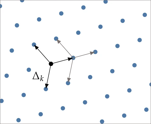
Figure 7.10:Meshing strategy extended across the domain. The same directions (and potentially spacing) are repeated at each mesh point, as indicated by the lighter arrows throughout the entire domain.
We describe one option for a search procedure based on the same mesh ideas as the polling step. The concept is to extend the mesh throughout the entire domain, as shown in Figure 7.10. In this example, the mesh size is shared between the search and poll phases. However, it is usually more effective if these sizes are independent. Mathematically, we can define the global mesh as the set
where is a matrix whose columns contain the basis vectors . The vector consists of nonnegative integers, and we consider all possible combinations of integers that fall within the bounds of the domain.
We choose a fixed number of search evaluation points and randomly select points from the global mesh for the search strategy. If improvement is found among that set, then we recenter at this improved point, grow the mesh (), and end the iteration (and then restart the search). A simple search phase along these lines is described in Algorithm 7.2 and the main GPS algorithm is shown in Algorithm 7.3.
The convergence of the GPS algorithm is often determined by a user-specified maximum number of iterations. However, other criteria are also used, such as a threshold on mesh size or a threshold on the improvement in the function value over previous iterations.
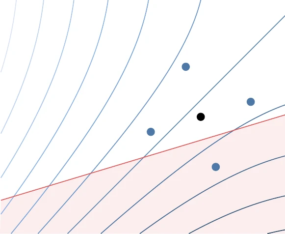
Figure 7.11:Mesh direction changed during optimization to align with linear constraints when close to the constraint.
GPS can handle linear and nonlinear constraints. For linear constraints, one effective strategy is to change the positive spanning directions so that they align with any linear constraints that are nearby (Figure 7.11). For nonlinear constraints, penalty approaches (Section 5.4) are applicable, although the filter method (Section 5.5.3) is another effective approach.
MADS is a well-known extension of GPS. The main difference between these two methods is in the number of possibilities for polling directions.8 In GPS, the polling directions are relatively restrictive (e.g., left side of Figure 7.13 for a minimal basis in two dimensions). MADS adds a new sizing parameter called the poll size parameter () that can be varied independently from the existing mesh size parameter (). These sizes are constrained by so the mesh sizing can become smaller while allowing the poll size (which dictates the maximum magnitude of the step) to remain large. This provides a much denser set of options in poll directions (e.g., the grid points on the right panel of Figure 7.13). MADS randomly chooses the polling directions from this much larger set of possibilities while maintaining a positive spanning set.[6]
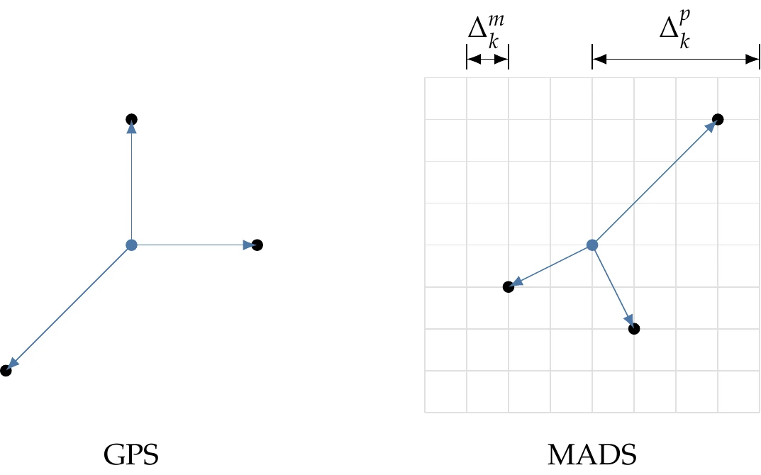
Figure 7.13:Typical GPS spanning directions (left). In contrast, MADS randomly selects from many potential spanning directions by utilizing a finer mesh (right).
7.5 DIRECT Algorithm
The DIRECT algorithm is different from the other gradient-free optimization algorithms in this chapter in that it is based on mathematical arguments.[7] This is a deterministic method guaranteed to converge to the global optimum under conditions that are not too restrictive (although it might require a prohibitive number of function evaluations). DIRECT has been extended to handle constraints without relying on penalty or filtering methods, but here we only explain the algorithm for unconstrained problems.12
One way to ensure that we find the global optimum within a finite design space is by dividing this space into a regular rectangular grid and evaluating every point in this grid. This is called an exhaustive search, and the precision of the minimum depends on how fine the grid is. The cost of this brute-force strategy is high and goes up exponentially with the number of design variables.
The DIRECT method relies on a grid, but it uses an adaptive meshing scheme that dramatically reduces the cost. It starts with a single -dimensional hypercube that spans the whole design space—like many other gradient-free methods, DIRECT requires upper and lower bounds on all the design variables. Each iteration divides this hypercube into smaller ones and evaluates the objective function at the center of each of these. At each iteration, the algorithm only divides rectangles determined to be potentially optimal. The fundamental strategy in the DIRECT method is how it determines this subset of potentially optimal rectangles, which is based on the mathematical concept of Lipschitz continuity.
We start by explaining Lipschitz continuity and then describe an algorithm for finding the global minimum of a one-dimensional function using this concept—Shubert’s algorithm. Although Shubert’s algorithm is not practical in general, it will help us understand the mathematical rationale for the DIRECT algorithm. Then we explain the DIRECT algorithm for one-dimensional functions before generalizing it for dimensions.
Lipschitz Constant
Consider the single-variable function shown in Figure 7.14. For a trial point , we can draw a cone with slope by drawing the lines
to the left and right, respectively. We show this cone in Figure 7.14 (left), as well as cones corresponding to other values of .
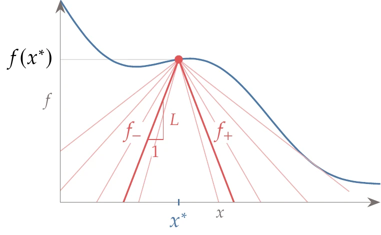
Figure 7.14:From a given trial point , we can draw a cone with slope (a). For a function to be Lipschitz continuous, we need all cones with slope to lie under the function for all points in the domain (b).
A function is said to be Lipschitz continuous if there is a cone slope such that the cones for all possible trial points in the domain remain under the function. This means that there is a positive constant such that
where is the function domain. Graphically, this condition means that we can draw a cone with slope from any trial point evaluation such that the function is always bounded by the cone, as shown in Figure 7.14 (right). Any that satisfies Equation 7.14 is a Lipschitz constant for the corresponding function.
Shubert’s Algorithm
If a Lipschitz constant for a single-variable function is known, Shubert’s algorithm can find the global minimum of that function. Because the Lipschitz constant is not available in the general case, the DIRECT algorithm is designed to not require this constant. However, we explain Shubert’s algorithm first because it provides some of the basic concepts used in the DIRECT algorithm.
Shubert’s algorithm starts with a domain within which we want to find the global minimum— in Figure 7.15. Using the property of the Lipschitz constant defined in Equation 7.14, we know that the function is always above a cone of slope evaluated at any point in the domain.
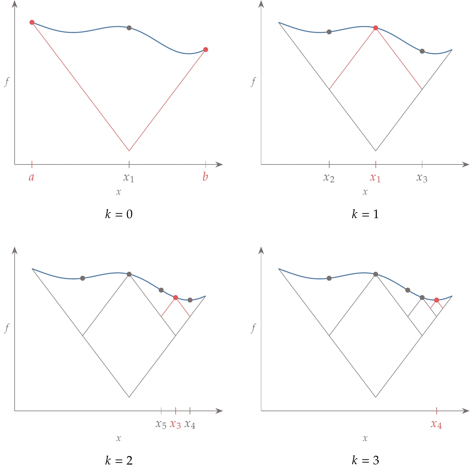
Figure 7.15:Shubert’s algorithm requires an initial domain and a valid Lipschitz constant and then increases the lower bound of the global minimum with each successive iteration.
Shubert’s algorithm starts by sampling the endpoints of the interval within which we want to find the global minimum ( in Figure 7.15). We start by establishing a first lower bound on the global minimum by finding the cone’s intersection ( in Figure 7.15, ) for the extremes of the domain. We evaluate the function at and can now draw a cone about this point to find two more intersections ( and ). Because these two points always intersect at the same objective lower bound value, they both need to be evaluated.
Each subsequent iteration of Shubert’s algorithm adds two new points to either side of the current point. These two points are evaluated, and the lower bounding function is updated with the resulting new cones. We then iterate by finding the two points that minimize the new lower bounding function, evaluating the function at these points, updating the lower bounding function, and so on.
The lowest bound on the function increases at each iteration and ultimately converges to the global minimum. At the same time, the segments in decrease in size. The lower bound can switch from distinct regions as the lower bound in one region increases beyond the lower bound in another region.
The two significant shortcomings of Shubert’s algorithm are that (1) a Lipschitz constant is usually not available for a general function, and (2) it is not easily extended to dimensions. The DIRECT algorithm addresses these two shortcomings.
One-Dimensional DIRECT
Before explaining the -dimensional DIRECT algorithm, we introduce the one-dimensional version based on principles similar to those of the Shubert algorithm.
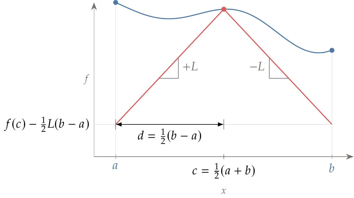
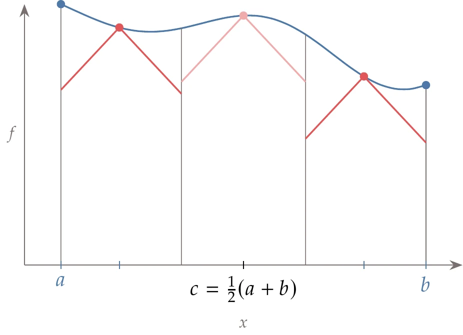
Figure 7.16:The DIRECT algorithm evaluates the middle point (a), and each successive iteration trisects the segments that have the greatest potential (b).
Like Shubert’s method, DIRECT starts with the domain . However, instead of sampling the endpoints and , it samples the midpoint. Consider the closed domain shown in Figure 7.16 (left). For each segment, we evaluate the objective function at the segment’s midpoint. In the first segment, which spans the whole domain, the midpoint is . Assuming some value of , which is not known and that we will not need, the lower bound on the minimum would be .
We want to increase this lower bound on the function minimum by dividing this segment further. To do this in a regular way that reuses previously evaluated points and can be repeated indefinitely, we divide it into three segments, as shown in Figure 7.16 (right). Now we have increased the lower bound on the minimum. Unlike the Shubert algorithm, the lower bound is a discontinuous function across the segments, as shown in Figure 7.16 (right).
Instead of continuing to divide every segment into three other segments, we only divide segments selected according to a potentially optimal criterion. To better understand this criterion, consider a set of segments at a given DIRECT iteration, where segment has a half-length and a function value evaluated at the segment center . If we plot versus for a set of segments, we get the pattern shown in Figure 7.17.
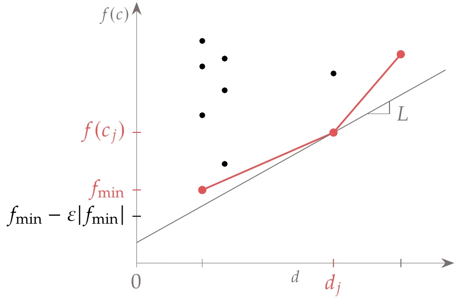
Figure 7.17:Potentially optimal segments in the DIRECT algorithm are identified by the lower convex hull of this plot.
The overall rationale for the potentially optimal criterion is that two metrics quantify this potential: the size of the segment and the function value at the center of the segment. The larger the segment is, the greater the potential for that segment to contain the global minimum. The lower the function value, the greater that potential is as well. For a set of segments of the same size, we know that the one with the lowest function value has the best potential and should be selected. If two segments have the same function value and different sizes, we should select the one with the largest size. For a general set of segments with various sizes and value combinations, there might be multiple segments that can be considered potentially optimal.
We identify potentially optimal segments as follows. If we draw a line with a slope corresponding to a Lipschitz constant from any point in Figure 7.17, the intersection of this line with the vertical axis is a bound on the objective function for the corresponding segment. Therefore, the lowest bound for a given can be found by drawing a line through the point that achieves the lowest intersection.
However, we do not know , and we do not want to assume a value because we do not want to bias the search. If were high, it would favor dividing the larger segments. Low values of would result in dividing the smaller segments. The DIRECT method hinges on considering all possible values of , effectively eliminating the need for this constant.
To eliminate the dependence on , we select all the points for which there is a line with slope that does not go above any other point.
This corresponds to selecting the points that form a lower convex hull, as shown by the piecewise linear function in Figure 7.17. This establishes a lower bound on the function for each segment size.
Mathematically, a segment in the set of current segments is said to be potentially optimal if there is a such that
where is the best current objective function value, and is a small positive parameter. The first condition corresponds to finding the points in the lower convex hull mentioned previously.
The second condition in Equation 7.16 ensures that the potential minimum is better than the lowest function value found so far by at least a small amount. This prevents the algorithm from becoming too local, wasting function evaluations in search of smaller function improvements. The parameter balances the search between local and global. A typical value is , and its range is usually such that .
There are efficient algorithms for finding the convex hull of an arbitrary set of points in two dimensions, such as the Jarvis march.13
These algorithms are more than we need because we only require the lower part of the convex hull, so the algorithms can be simplified for our purposes.
As in the Shubert algorithm, the division might switch from one part of the domain to another, depending on the new function values. Compared with the Shubert algorithm, the DIRECT algorithm produces a discontinuous lower bound on the function values, as shown in Figure 7.18.
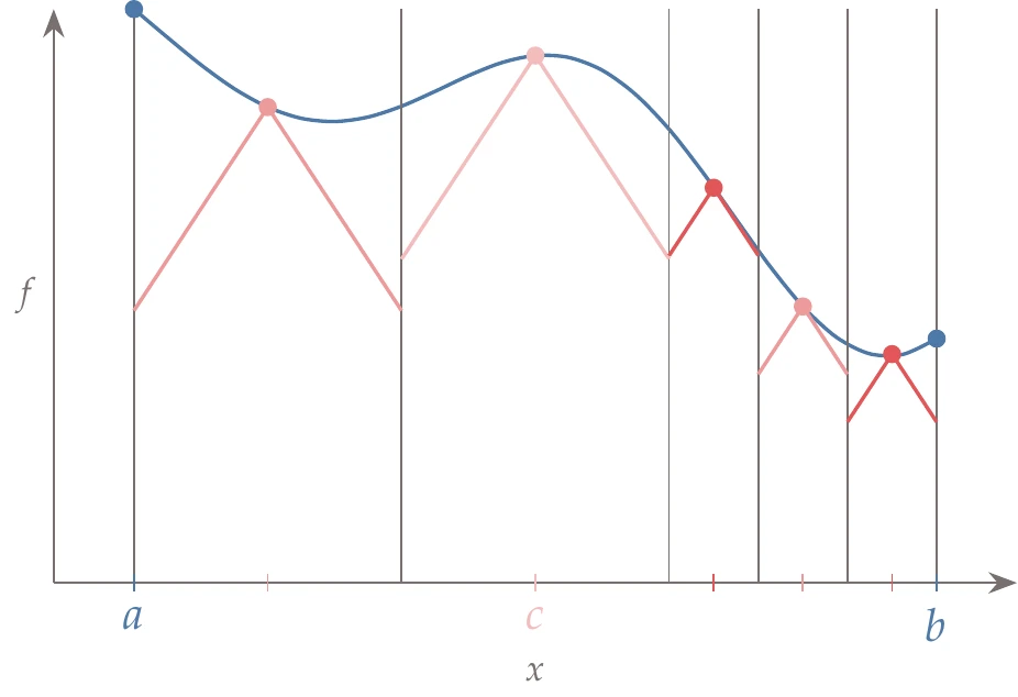
Figure 7.18:The lower bound for the DIRECT method is discontinuous at the segment boundaries.
DIRECT in Dimensions
The -dimensional DIRECT algorithm is similar to the one-dimensional version but becomes more complex.[8] The main difference is that we deal with hyperrectangles instead of segments. A hyperrectangle can be defined by its center-point position in -dimensional space and a half-length in each direction , , as shown in Figure 7.19. The DIRECT algorithm assumes that the initial dimensions are normalized so that we start with a hypercube.
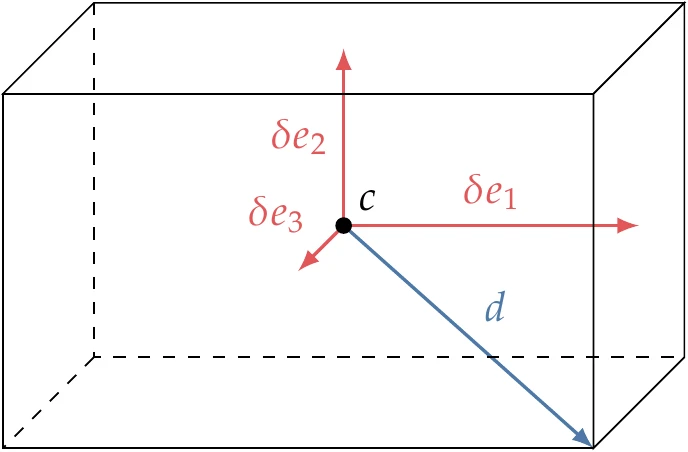
Figure 7.19:Hyperrectangle in three dimensions, where is the maximum distance between the center and the vertices, and is the half-length in each direction .
To identify the potentially optimal rectangles at a given iteration, we use exactly the same conditions in Equation 7.15 and Equation 7.16, but is now the center of the hyperrectangle, and is the maximum distance from the center to a vertex. The explanation illustrated in Figure 7.17 still applies in the -dimensional case and still involves simply finding the lower convex hull of a set of points with different combinations of and .
The main complication introduced in the -dimensional case is the division (trisection) of a selected hyperrectangle.
The question is which directions should be divided first. The logic to handle this in the DIRECT algorithm is to prioritize reducing the dimensions with the maximum length, ensuring that hyperrectangles do not deviate too much from the proportions of a hypercube. First, we select the set of the longest dimensions for division (there are often multiple dimensions with the same length).
Among this set of the longest dimensions, we select the direction that has been divided the least over the whole history of the search. If there are still multiple dimensions in the selection, we simply select the one with the lowest index. Algorithm 7.4 details the full algorithm.[9]
Figure 7.20 shows the first three iterations for a two-dimensional example and the corresponding visualization of the conditions expressed in Equation 7.15 and Equation 7.16. We start with a square that contains the whole domain and evaluate the center point. The value of this point is plotted on the – plot on the far right.
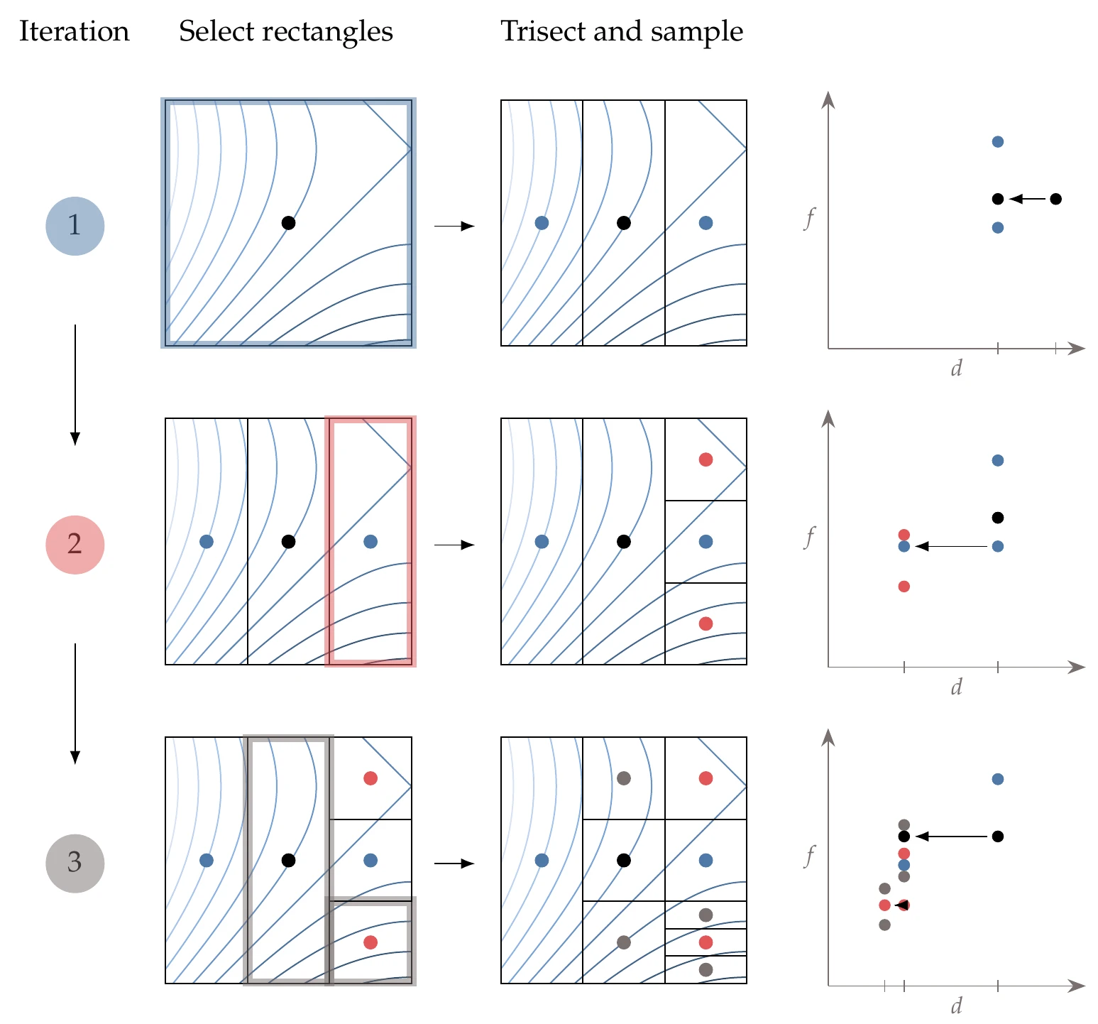
Figure 7.20:DIRECT iterations for two-dimensional case (left) and corresponding identification of potentially optimal rectangles (right).
The first iteration trisects the starting square along the first dimension and evaluates the two new points. The values for these three points are plotted in the second column from the right in the – plot, where the center point is reused, as indicated by the arrow and the matching color. At this iteration, we have two points that define the convex hull.
In the second iteration, we have three rectangles of the same size, so we divide the one with the lowest value and evaluate the centers of the two new rectangles (which are squares in this case). We now have another column of points in the – plot corresponding to a smaller and an additional point that defines the lower convex hull. Because the convex hull now has two points, we trisect two different rectangles in the third iteration.
7.6 Genetic Algorithms
Genetic algorithms (GAs) are the most well-known and widely used type of evolutionary algorithm. They were also among the earliest to have been developed.[10]
Like many evolutionary algorithms, GAs are population based. The optimization starts with a set of design points (the population) rather than a single starting point, and each optimization iteration updates this set in some way. Each GA iteration is called a generation, each of which has a population with points. Each point is represented by a chromosome, which contains the values for all the design variables, as shown in Figure 7.23. Each design variable is represented by a gene. As we will see later, there are different ways for genes to represent the design variables.
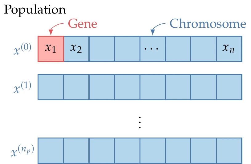
Figure 7.23:Each GA iteration involves a population of design points, where each design is represented by a chromosome, and each design variable is represented by a gene.
GAs evolve the population using an algorithm inspired by biological reproduction and evolution using three main steps: (1) selection, (2) crossover, and (3) mutation. Selection is based on natural selection, where members of the population that acquire favorable adaptations are more likely to survive longer and contribute more to the population gene pool. Crossover is inspired by chromosomal crossover, which is the exchange of genetic material between chromosomes during sexual reproduction.
Mutation mimics genetic mutation, which is a permanent change in the gene sequence that occurs naturally.
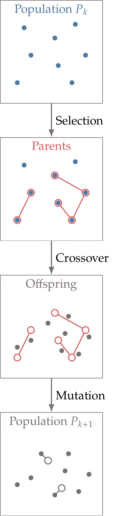
Figure 7.24:GA iteration steps.
Algorithm 7.5 and Figure 7.24 show how these three steps perform optimization. Although most GAs follow this general procedure, there is a great degree of flexibility in how the steps are performed, leading to many variations in GAs. For example, there is no single method specified for the generation of the initial population, and the size of that population varies. Similarly, there are many possible methods for selecting the parents, generating the offspring, and selecting the survivors. Here, the new population () is formed exclusively by the offspring generated from the crossover. However, some GAs add an extra selection process that selects a surviving population of size among the population of parents and offspring.
In addition to the flexibility in the various operations, GAs use different methods for representing the design variables. The design variable representation can be used to classify genetic algorithms into two broad categories: binary-encoded and real-encoded genetic algorithms. Binary-encoded algorithms use bits to represent the design variables, whereas the real-encoded algorithms keep the same real value representation used in most other algorithms. The details of the operations in Algorithm 7.5 depend on whether we are using one or the other representation, but the principles remain the same. In the rest of this section, we describe a particular way of performing these operations for each of the possible design variable representations.
7.6.1 Binary-Encoded Genetic Algorithms
The original genetic algorithms were based on binary encoding because they more naturally mimic chromosome encoding. Binary-coded GAs are applicable to discrete or mixed-integer problems.[11] When using binary encoding, we represent each variable as a binary number with bits. Each bit in the binary representation has a location, , and a value, (which is either 0 or 1). If we want to represent a real-valued variable, we first need to consider a finite interval , which we can then divide into intervals. The size of the interval is given by
To have a more precise representation, we must use more bits.
When using binary-encoded GAs, we do not need to encode the design variables because they are generated and manipulated directly in the binary representation. Still, we do need to decode them before providing them to the evaluation function.
To decode a binary representation, we use
Initial Population
The first step in a genetic algorithm is to generate an initial set (population) of points. As a rule of thumb, the population size should be approximately one order of magnitude larger than the number of design variables, and this size should be tuned.
One popular way to choose the initial population is to do it at random. Using binary encoding, we can assign each bit in the representation of the design variables a 50 percent chance of being either 1 or 0. This can be done by generating a random number and setting the bit to 0 if and 1 if .
For a population of size , with design variables, where each variable is encoded using bits, the total number of bits that needs to be generated is .
To achieve better spread in a larger dimensional space, the sampling methods described in Section 10.2 are generally more effective than random populations.
Although we then need to evaluate the function across many points (a population), these evaluations can be performed in parallel.
Selection
In this step, we choose points from the population for reproduction in a subsequent step (called a mating pool). On average, it is desirable to choose a mating pool that improves in fitness (thus mimicking the concept of natural selection), but it is also essential to maintain diversity. In total, we need to generate pairs.
The simplest selection method is to randomly select two points from the population until the requisite number of pairs is complete. This approach is not particularly effective because there is no mechanism to move the population toward points with better objective functions.
Tournament selection is a better method that randomly pairs up points and selects the best point from each pair to join the mating pool. The same pairing and selection process is repeated to create more points to complete a mating pool of points.
Another standard method is roulette wheel selection. This concept is patterned after a roulette wheel used in a casino. Better points are allocated a larger sector on the roulette wheel to have a higher probability of being selected.
First, the objective function for all the points in the population must be converted to a fitness value because the roulette wheel needs all positive values and is based on maximizing rather than minimizing. To achieve that, we first perform the following conversion to fitness:
where is based on the highest and lowest function values in the population, and the denominator is introduced to scale the fitness.
Then, to find the sizes of the sectors in the roulette wheel selection, we take the normalized cumulative sum of the scaled fitness values to compute an interval for each member in the population as
We can now create a mating pool of points by turning the roulette wheel times. We do this by generating a random number at each turn. The member is copied to the mating pool if
This ensures that the probability of a member being selected for reproduction is proportional to its scaled fitness value.
Crossover
In the reproduction operation, two points (offspring) are generated from a pair of points (parents). Various strategies are possible in genetic algorithms. Single-point crossover usually involves generating a random integer that defines the crossover point. This is illustrated in Figure 7.27. For one of the offspring, the first bits are taken from parent 1 and the remaining bits from parent 2. For the second offspring, the first bits are taken from parent 2 and the remaining ones from parent 1. Various extensions exist, such as two-point crossover or -point crossover.
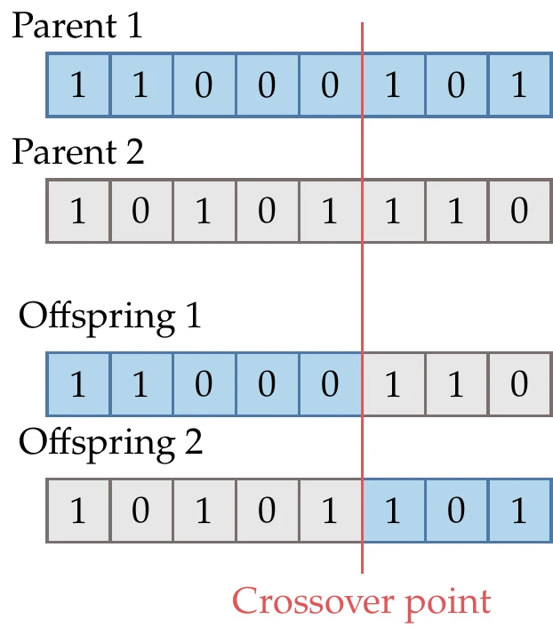
Figure 7.27:The crossover point determines which parts of the chromosome from each parent get inherited by each offspring.
Mutation
Mutation is a random operation performed to change the genetic information and is needed because even though selection and reproduction effectively recombine existing information, occasionally some useful genetic information might be lost. The mutation operation protects against such irrecoverable loss and introduces additional diversity into the population.
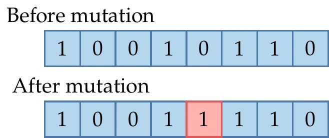
Figure 7.28:Mutation randomly switches some of the bits with low probability.
When using bit representation, every bit is assigned a small permutation probability, say . This is done by generating a random number for each bit, which is changed if . An example is illustrated in Figure 7.28.
7.6.2 Real-Encoded Genetic Algorithms
As the name implies, real-encoded GAs represent the design variables in their original representation as real numbers. This has several advantages over the binary-encoded approach. First, real encoding represents numbers up to machine precision rather than being limited by the number of bits chosen for the binary encoding. Second, it avoids the “Hamming cliff” issue of binary encoding, which is caused by the fact that many bits must change to move between adjacent real numbers (e.g., 0111 to 1000). Third, some real-encoded GAs can generate points outside the design variable bounds used to create the initial population; in many problems, the design variables are not bounded.
Finally, it avoids the burden of binary coding and decoding.
The main disadvantage is that integer or discrete variables cannot be handled. For continuous problems, a real-encoded GA is generally more efficient than a binary-encoded GA.6 We now describe the required changes to the GA operations in the real-encoded approach.
Initial Population
The most common approach is to pick the points using random sampling within the provided design bounds. Each member is often chosen at random within some initial bounds. For each design variable , with bounds such that , we could use,
where is a random number such that . Again, the sampling methods described in Section 10.2 are more effective for higher-dimensional spaces.
Selection
The selection operation does not depend on the design variable encoding. Therefore, we can use one of the selection approaches described for the binary-encoded GA: tournament or roulette wheel selection.
Crossover
When using real encoding, the term crossover does not accurately describe the process of creating the two offspring from a pair of points.
Instead, the approaches are more accurately described as a blending, although the name crossover is still often used.
There are various options for the reproduction of two points encoded using real numbers. A standard method is linear crossover, which generates two or more points in the line defined by the two parent points. One option for linear crossover is to generate the following two points:
where parent 2 is more fit than parent 1 ().
An example of this linear crossover approach is shown in Figure 7.29, where we can see that child 1 is the average of the two parent points, whereas child 2 is obtained by extrapolating in the direction of the “fitter” parent.
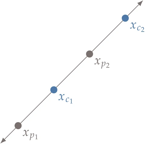
Figure 7.29:Linear crossover produces two new points along the line defined by the two parent points.
Another option is a simple crossover like the binary case where a random integer is generated to split the vectors—for example, with a split after the first index:
This simple crossover does not generate as much diversity as the binary case and relies more heavily on effective mutation. Many other strategies have been devised for real-encoded GAs.Deb (2001, Ch. 4)
Mutation
As with a binary-encoded GA, mutation should only occur with a small probability (e.g., ). However, rather than changing each bit with probability , we now change each design variable with probability .
Many mutation methods rely on random variations around an existing member, such as a uniform random operator:
where is a random number between 0 and 1, and is a preselected maximum perturbation in the th direction. Many nonuniform methods exist as well. For example, we can use a normal probability distribution
where is a preselected standard deviation, and random samples are drawn from the normal distribution. During the mutation operations, bound checking is necessary to ensure the mutations stay within the lower and upper limits.
7.6.3 Constraint Handling
Various approaches exist for handling constraints. Like the Nelder–Mead method, we can use a penalty method (e.g., augmented Lagrangian, linear penalty). However, there are additional options for GAs. In the tournament selection, we can use other selection criteria that do not depend on penalty parameters. One such approach for choosing the best selection among two competitors is as follows:
Prefer a feasible solution.
Among two feasible solutions, choose the one with a better objective.
Among two infeasible solutions, choose the one with a smaller constraint violation.
This concept is a lot like the filter methods discussed in Section 5.5.3.
7.6.4 Convergence
Rigorous mathematical convergence criteria, like those used in gradient-based optimization, do not apply to GAs. The most common way to terminate a GA is to specify a maximum number of iterations, which corresponds to a computational budget. Another similar approach is to let the algorithm run indefinitely until the user manually terminates the algorithm, usually by monitoring the trends in population fitness.
A more automated approach is to track a running average of the population’s fitness. However, it can be challenging to decide what tolerance to apply to this criterion because we generally are not interested in the average performance. A more direct metric of interest is the fitness of the best member in the population. However, this can be a problematic criterion because the best member can disappear as a result of crossover or mutation. To avoid this and to improve convergence, many GAs employ elitism. This means that the fittest population member is retained to guarantee that the population does not regress. Even without this behavior, the best member often changes slowly, so the user should not terminate the algorithm unless the best member has not improved for several generations.
7.7 Particle Swarm Optimization
Like a GA, particle swarm optimization (PSO) is a stochastic population-based optimization algorithm based on the concept of “swarm intelligence”. Swarm intelligence is the property of a system whereby the collective behaviors of unsophisticated agents interacting locally with their environment cause coherent global patterns. In other words: dumb agents, properly connected into a swarm, can yield smart results.[12]
The “swarm” in PSO is a set of design points (agents or particles) that move in -dimensional space, looking for the best solution. Although these are just design points, the history for each point is relevant to the PSO algorithm, so we adopt the term particle. Each particle moves according to a velocity. This velocity changes according to the past objective function values of that particle and the current objective values of the rest of the particles. Each particle remembers the location where it found its best result so far, and it exchanges information with the swarm about the location where the swarm has found the best result so far.
The position of particle for iteration is updated according to
where is a constant artificial time step. The velocity for each particle is updated as follows:
The first component in this update is the “inertia”, which determines how similar the new velocity is to the velocity in the previous iteration through the parameter . Typical values for the inertia parameter are in the interval .
A lower value of reduces the particle’s inertia and tends toward faster convergence to a minimum. A higher value of increases the particle’s inertia and tends toward increased exploration to potentially help discover multiple minima. Some methods are adaptive, choosing the value of based on the optimizer’s progress.20
The second term represents “memory” and is a vector pointing toward the best position particle has seen in all its iterations so far, . The weight in this term consists of a random number in the interval that introduces a stochastic component to the algorithm. Thus, controls how much influence the best point found by the particle so far has on the next direction.
The third term represents “social” influence. It behaves similarly to the memory component, except that is the best point the entire swarm has found so far, and is a random number between that controls how much of an influence this best point has in the next direction. The relative values of and thus control the tendency toward local versus global search, respectively. Both and are in the interval and are typically closer to 2. Sometimes, rather than using the best point in the entire swarm, the best point is chosen within a neighborhood.
Because the time step is artificial, we can eliminate it by multiplying Equation 7.28 by to yield a step:
We then use this step to update the particle position for the next iteration:
The three components of the update in Equation 7.29 are shown in Figure 7.32 for a two-dimensional case.
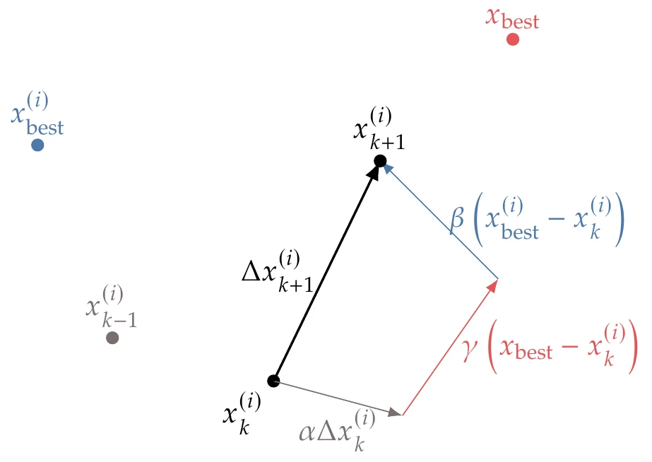
Figure 7.32:Components of the PSO update.
The first step in the PSO algorithm is to initialize the set of particles (Algorithm 7.6). As with a GA, the initial set of points can be determined randomly or can use a more sophisticated sampling strategy (see Section 10.2). The velocities are also randomly initialized, generally using some fraction of the domain size ().
The main loop in the algorithm computes the steps to be added to each particle and updates their positions. Particles must be prevented from going beyond the bounds. If a particle reaches a boundary and has a velocity pointing out of bounds, it is helpful to reset to velocity to zero or reorient it toward the interior for the next iteration. It is also helpful to impose a maximum velocity. If the velocity is too large, the updated positions are unrelated to their previous positions, and the search is more random. The maximum velocity might also decrease across iterations to shift from exploration toward exploitation.
Several convergence criteria are possible, some of which are similar to the Nelder–Mead algorithm and GAs. Examples of convergence criteria include the distance (sum or norm) between each particle and the best particle, the best particle’s objective function value changes for the last few generations, and the difference between the best and worst member. For PSO, another alternative is to check whether the velocities for all particles (as measured by a metric such as norm or mean) are below some tolerance. Some of these criteria that assume all the particles congregate (distance, velocities) do not work well for multimodal problems. In those cases, tracking only the best particle’s objective function value may be more appropriate.
7.8 Summary
Gradient-free optimization algorithms are needed when the objective and constraint functions are not smooth enough or when it is not possible to compute derivatives with enough precision. One major advantage of gradient-free methods is that they tend to be robust to numerical noise and discontinuities, making them easier to use than gradient-based methods.
However, the overall cost of gradient-free optimization is sensitive to the cost of the function evaluations because they require many iterations for convergence, and the number of iterations scales poorly with the number of design variables.
There is a wide variety of gradient-free methods. They can perform a local or global search, use mathematical or heuristic criteria, and be deterministic or stochastic. A global search does not guarantee convergence to the global optimum but increases the likelihood of such convergence. We should be wary when heuristics establish convergence because the result might not correspond to the actual mathematical optimum. Heuristics in the optimization algorithm also limit the rate of convergence compared with algorithms based on mathematical principles.
In this chapter, we covered only a small selection of popular gradient-free algorithms. The Nelder–Mead algorithm is a local search algorithm based on heuristics and is easy to implement. GPS and DIRECT are based on mathematical criteria.
Evolutionary algorithms are global search methods based on the evolution of a population of designs. They stem from appealing heuristics inspired by natural or societal phenomena and have some stochastic element in their algorithms. The GAs and PSO algorithms covered in this chapter are only two examples from the plethora of evolutionary algorithms that have been invented.
Many of the methods presented in this chapter do not directly address constrained problems; in those cases, penalty or filtering methods are typically used to enforce constraints.
Problems
6 provides a more comprehensive review of evolutionary algorithms.
These algorithms include the following: ant colony optimization, artificial bee colony algorithm, artificial fish swarm, artificial flora optimization algorithm, bacterial foraging optimization, bat algorithm, big bang–big crunch algorithm, biogeography-based optimization, bird mating optimizer, cat swarm optimization, cockroach swarm optimization, cuckoo search, design by shopping paradigm, dolphin echolocation algorithm, elephant herding optimization, firefly algorithm, flower pollination algorithm, fruit fly optimization algorithm, galactic swarm optimization, gray wolf optimizer, grenade explosion method, harmony search algorithm, hummingbird optimization algorithm, hybrid glowworm swarm optimization algorithm, imperialist competitive algorithm, intelligent water drops, invasive weed optimization, mine bomb algorithm, monarch butterfly optimization, moth-flame optimization algorithm, penguin search optimization algorithm, quantum-behaved particle swarm optimization, salp swarm algorithm, teaching–learning-based optimization, whale optimization algorithm, and water cycle algorithm.
Section 5.2n-Dimensional Space discusses the concept of span and polyhedral cones; Figure 5.6 is particularly relevant.
Algorithm 7.4 follows the revised version of DIRECT,12 which differs from the original version.14 The original version trisected all the long sides of the selected rectangles instead of just one side.
The first GA software was written in 1954, followed by other seminal work.15 Initially, these GAs were not developed to perform optimization but rather to model the evolutionary process. GAs were eventually applied to optimization.16
One popular binary-encoded genetic algorithm implementation is the elitist nondominated sorting genetic algorithm (NSGA-II; discussed in Section 9.3.4 in connection with multiobjective optimization).17
- Yu, Y., Lyu, Z., Xu, Z., & Martins, J. R. R. A. (2018). On the influence of optimization algorithm and starting design on wing aerodynamic shape optimization. Aerospace Science and Technology, 75, 183–199. 10.1016/j.ast.2018.01.016
- Rios, L. M., & Sahinidis, N. V. (2013). Derivative-free optimization: a review of algorithms and comparison of software implementations. Journal of Global Optimization, 56, 1247–1293. 10.1007/s10898-012-9951-y
- Conn, A. R., Scheinberg, K., & Vicente, L. N. (2009). Introduction to Derivative-Free Optimization. SIAM. 10.1137/1.9780898718768
- Audet, C., & Hare, W. (2017). Derivative-Free and Blackbox Optimization. Springer. 10.1007/978-3-319-68913-5
- Kokkolaras, M. (2020). When, why, and how can derivative-free optimization be useful to computational engineering design? Journal of Mechanical Design, 142(1), 010301. 10.1115/1.4045043
- Simon, D. (2013). Evolutionary Optimization Algorithms. John Wiley & Sons.
- Nelder, J. A., & Mead, R. (1965). A simplex method for function minimization. Computer Journal, 7, 308–313. 10.1093/comjnl/7.4.308
- Audet, C., & J. E. Dennis, J. (2006). Mesh adaptive direct search algorithms for constrained optimization. SIAM Journal on Optimization, 17(1), 188–217. 10.1137/040603371
- Le Digabel, S. (2011). Algorithm 909: NOMAD: Nonlinear optimization with the MADS algorithm. ACM Transactions on Mathematical Software, 37(4), 1–15. 10.1145/1916461.1916468
- Jones, D. R., Perttunen, C. D., & Stuckman, B. E. (1993). Lipschitzian optimization without the Lipschitz constant. Journal of Optimization Theory and Application, 79(1), 157–181. 10.1007/BF00941892
- Jones, D. R., & Martins, J. R. R. A. (2021). The DIRECT algorithm—25 years later. Journal of Global Optimization, 79, 521–566. 10.1007/s10898-020-00952-6
- Jones, D. R. (2009). Direct Global Optimization Algorithm. In C. A. Floudas & P. M. Pardalos (Eds.), Encyclopedia of Optimization (pp. 725–735). Springer. 10.1007/978-0-387-74759-0_128
- Jarvis, R. A. (1973). On the identification of the convex hull of a finite set of points in the plane. Information Processing Letters, 2(1), 18–21. 10.1016/0020-0190(73)90020-3
- Jones, D. R., Schonlau, M., & Welch, W. J. (1998). Efficient global optimization of expensive black-box functions. Journal of Global Optimization, 13, 455–492. 10.1023/A:1008306431147
- Barricelli, N. (1954). Esempi numerici di processi di evoluzione. Methodos, 45–68.