Numerical Models and Solvers - Engineering Design Optimization

In the introductory chapter, we discussed function characteristics from the point of view of the function’s output—the black-box view shown in Figure 1.16. Here, we discuss how the function is modeled and computed. The better your understanding of the model and the more access you have to its details, the more effectively you can solve the optimization problem. We explain the errors involved in the modeling process so that we can interpret optimization results correctly.

3.1 Model Development for Analysis versus Optimization¶

A good understanding of numerical models and solvers is essential because numerical optimization demands more from the models and solvers than does pure analysis. In an analysis or a parametric study, we may cycle through a range of plausible designs. However, optimization algorithms seek to explore the design space, and therefore, intermediate evaluations may use atypical design variables combinations. The mathematical model, numerical model, and solver must be robust enough to handle these design variable combinations.

A related issue is that an optimizer exploits errors in ways an engineer would not do in analysis. For example, consider the aerodynamic analysis of a car. In a parametric study, we might try a dozen designs, compare the drag, and choose the best one. If we passed this procedure to an optimizer, it might flatten the car to zero height (the minimum drag solution) if there are no explicit constraints on interior volume or structural integrity. Thus, we often need to develop additional models for optimization. A designer often considers some of these requirements implicitly and approximately, but we need to model these requirements explicitly and pose them as constraints in optimization.

Another consideration that affects both the mathematical and the numerical model is the overall computational cost of optimization. An analysis might only be run dozens of times, whereas an optimization often runs the analysis thousands of times. This computational cost can affect the level of fidelity or discretization we can afford to use.

The level of precision desirable for analysis is often insufficient for optimization. In an analysis, a few digits of precision may be sufficient. However, using fewer significant digits limits the types of optimization algorithms we can employ effectively. Convergence failures can cause premature termination of algorithms. Noisy outputs can mislead or terminate an optimization prematurely. A common source of these errors involves programs that work through input and output files (see Tip 6.1). Even though the underlying code may use double-precision arithmetic, output files rarely include all the significant digits (another separate issue is that reading and writing files at every iteration considerably slows down the analysis).

Another common source of errors involves converging systems of equations, as discussed later in this chapter. Optimization generally requires tighter tolerances than are used for analysis. Sometimes this is as easy as changing a default tolerance, but other times we need to rethink the solvers.

3.2 Modeling Process and Types of Errors¶

Design optimization problems usually involve modeling a physical system to compute the objective and constraint function values for a given design. Figure 3.1 shows the steps in the modeling process. Each of these steps in the modeling process introduces errors.

The physical system represents the reality that we want to model. The mathematical model can range from simple mathematical expressions to continuous differential or integral equations for which closed-form solutions over an arbitrary domain are not possible. Modeling errors are introduced in the idealizations and approximations performed in the derivation of the mathematical model. The errors involved in the rest of the process are numerical errors, which we detail in Section 3.5. In Section 3.3, we discuss mathematical models in more detail and establish the notation for representing them.

When a mathematical model is given by differential or integral equations, we must discretize the continuous equations to obtain the numerical model. Section 3.4 provides a brief overview of the discretization process, and Section 3.5.2 defines the associated errors.

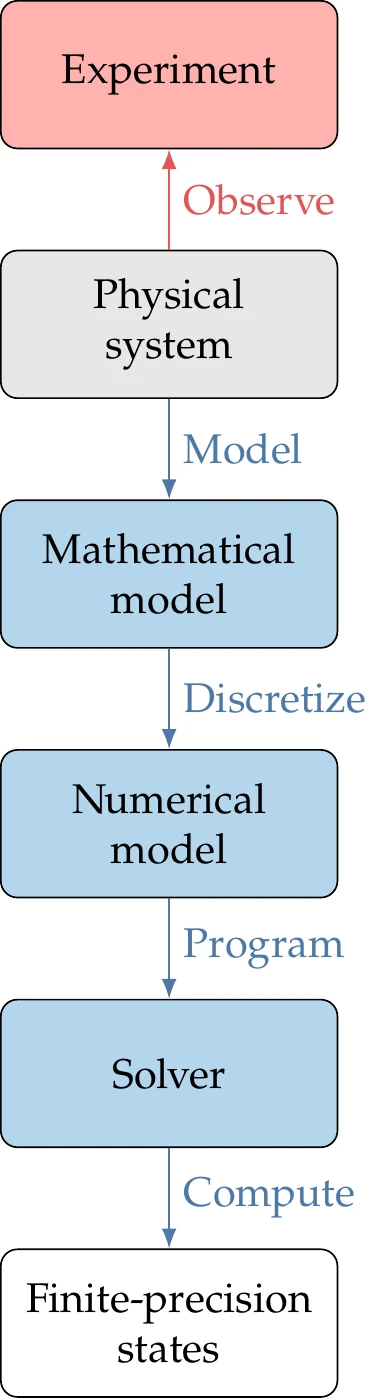
Figure 3.1:Physical problems are modeled and then solved numerically to produce function values.

The numerical model must then be programmed using a computer language to develop a numerical solver. Because this process is susceptible to human error, we discuss strategies for addressing such errors in Section 3.5.4.

Finally, the solver computes the system state variables using finite-precision arithmetic, which introduces roundoff errors (see Section 3.5.1). Section 3.6 includes a brief overview of solvers, and we dedicate a separate section to Newton-based solvers in Section 3.8 because they are used later in this book.

The total error in the modeling process is the sum of the modeling errors and numerical errors. Validation and verification processes quantify and reduce these errors. Verification ensures that the model and solver are correctly implemented so that there are no errors in the code. It also ensures that the errors introduced by discretization and numerical computations are acceptable. Validation compares the numerical results with experimental observations of the physical system, which are themselves subject to experimental errors. By making these comparisons, we can validate the modeling step of the process and ensure that the mathematical model idealizations and assumptions are acceptable.

Modeling and numerical errors relate directly to the concepts of precision and accuracy. An accurate solution compares well with the actual physical system (validation), whereas a precise solution means that the model is programmed and solved correctly (verification).

It is often said that “all models are wrong, but some are useful”.1 Because there are always errors involved, we must prioritize which aspects of a given model should be improved to reduce the overall error. When developing a new model, we should start with the simplest model that includes the system’s dominant behavior. Then, we might selectively add more detail as needed. One common pitfall in numerical modeling is to confuse precision with accuracy. Increasing precision by reducing the numerical errors is usually desirable. However, when we look at the bigger picture, the model might have limited utility if the modeling errors are more significant than the numerical errors.

Example 3.1 (Modeling a structure)

Figure 3.2:Timber roof truss and idealized model.

As an example of a physical system, consider the timber roof truss structure shown in Figure 3.2. A typical mathematical model of such a structure idealizes the wood as a homogeneous material and the joints as pinned. It is also common to assume that the loads are applied only at the joints and that the structure’s weight does not contribute to the loading. Finally, the displacements are assumed to be small relative to the dimensions of the truss members. The structure is discretized by pinned bar elements. The discrete governing equations for any truss structure can be derived using the finite-element method. This leads to the linear system

K u = q \, ,

where $K$ is the stiffness matrix, $q$ is the vector of applied loads, and $u$ represents the displacements that we want to compute. At each joint, there are two degrees of freedom (horizontal and vertical) that describe the displacement and applied force. Because there are 9 joints, each with 2 degrees of freedom, the size of this linear system is 18.

3.3 Numerical Models as Residual Equations¶

Mathematical models vary significantly in complexity and scale. In the simplest case, a model can be represented by one or more explicit functions, which are easily coded and computed. Many examples in this book use explicit functions for simplicity. In practice, however, many numerical models are defined by implicit equations.

Implicit equations can be written in the residual form as

r_i(u_1, \ldots, u_n) = 0, \quad i=1,\ldots, n \, ,

(3.1)

where $r$ is a vector of residuals that has the same size as the vector of state variables $u$ . The equations defining the residuals could be any expression that can be coded in a computer program. No matter how complex the mathematical model, it can always be written as a set of equations in this form, which we write more compactly as $r(u)=0$ .

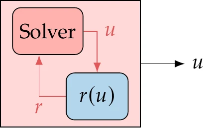
Numerical models use a solver to find the state variables u that satisfy the governing equations, such that r(u)=0. — Figure 3.3:Numerical models use a solver to find the state variables $u$ that satisfy the governing equations, such that $r(u)=0$ .

Finding the state variables that satisfy this set of equations requires a solver, as illustrated in Figure 3.3. We review the various types of solvers in Section 3.6. Solving a set of implicit equations is more costly than computing explicit functions, and it is typically the most expensive step in the optimization cycle.

Mathematical models are often referred to as governing equations, which determine the state ( $u$ ) of a given physical system at specific conditions. Many governing equations consist of differential equations, which require discretization. The discretization process yields implicit equations that can be solved numerically (see Section 3.4). After discretization, the governing equations can always be written as a set of residuals, $r(u)=0$ .

Example 3.2 (Implicit and explicit equations in structural analysis)

The linear system from Example 3.1 is an example of a system of implicit equations, which we can write as a set of residuals by moving the right-hand-side vector to the left to obtain

r(u) = Ku-q = 0 \, ,

where $u$ represents the state variables. Although the solution for $u$ could be written as an explicit function, $u = K^{-1}f$ , this is usually not done because it is computationally inefficient and intractable for large-scale systems. Instead, we use a linear solver that does not explicitly form the inverse of the stiffness matrix (see ).

In addition to computing the displacements, we might also want to compute the axial stress ( $\sigma$ ) in each of the 15 truss members.

This is an explicit function of the displacements, which is given by the linear relationship

\sigma = S u \, ,

where $S$ is a $(15 \times 18)$ matrix.

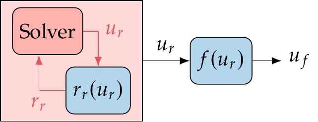
Figure 3.4:A model with implicit and explicit functions.

We can still use the residual notation to represent explicit functions to write all the functions in a model (implicit and explicit) as $r(u)=0$ without loss of generality. Suppose we have an implicit system of equations, $r_r(u_r)=0$ , followed by a set of explicit functions whose output is a vector $u_f = f(u_r)$ , as illustrated in Figure 3.4. We can rewrite the explicit function as a residual by moving all the terms to one side to get $r_f(u_r,u_f) = f(u_r) - u_f=0$ . Then, we can concatenate the residuals and variables for the implicit and explicit equations as

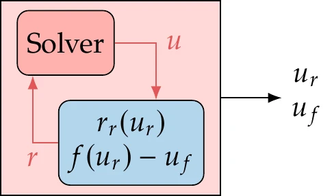
Figure 3.5:Explicit functions can be written in residual form and added to the solver.

r(u) \equiv \begin{bmatrix} r_r(u_r) \\ f(u_r) - u_f \end{bmatrix} = \begin{bmatrix} 0 \\ 0 \end{bmatrix} \, , \quad \text{where} \quad u \equiv \begin{bmatrix} u_r \\ u_f \end{bmatrix} \, .

(3.2)

The solver arrangement would then be as shown in Figure 3.5.

Even though it is more natural to just evaluate explicit functions instead of adding them to a solver, in some cases, it is helpful to use the residual to represent the entire model with the compact notation, $r(u)=0$ . This will be helpful in later chapters when we compute derivatives (Chapter 6) and solve systems that mix multiple implicit and explicit sets of equations (Chapter 13).

Example 3.3 (Expressing an explicit function as an implicit equation)

Suppose we have the following mathematical model:

\begin{aligned} u_1^2 + 2 u_2 - 1 &= 0 \\ u_1 + \cos (u_1) - u_2 &= 0 \\ f(u_1, u_2) &= u_1 + u_2 \, . \end{aligned}

The first two equations are written in implicit form, and the third equation is given as an explicit function. The first equation could be manipulated to obtain an explicit function of either $u_1$ or $u_2$ . The second equation does not have a closed-form solution and cannot be written as an explicit function for $u_1$ . The third equation is an explicit function of $u_1$ and $u_2$ . In this case, we could solve the first two equations for $u_1$ and $u_2$ using a nonlinear solver and then evaluate $f(u_1, u_2)$ . Alternatively, we can write the whole system as implicit residual equations by defining the value of $f(u_1, u_2)$ as $u_3$ ,

\begin{aligned} r_1(u_1, u_2) &= u_1^2 + 2 u_2 - 1 &= 0 \\ r_2(u_1, u_2) &= u_1 + \cos (u_1) - u_2 &= 0 \\ r_3(u_1, u_2, u_3) &= u_1 + u_2 - u_3 &= 0 &\, . \end{aligned}

Then we can use the same nonlinear solver to solve for all three equations simultaneously.

3.4 Discretization of Differential Equations¶

Many physical systems are modeled by differential equations defined over a domain. The domain can be spatial (one or more dimensions), temporal, or both. When time is considered, then we have a dynamic model. When a differential equation is defined in a domain with one degree of freedom (one-dimensional in space or time), then we have an ordinary differential equation (ODE), whereas any domain defined by more than one variable results in a partial differential equation (PDE).

Differential equations need to be discretized over the domain to be solved numerically. There are three main methods for the discretization of differential equations: the finite-difference method, the finite-volume method, and the finite-element method. The finite-difference method approximates the derivatives in the differential equations by the value of the relevant quantities at a discrete number of points in a mesh (see Figure 3.6).

The finite-volume method is based on the integral form of the PDEs. It divides the domain into control volumes called cells (which also form a mesh), and the integral is evaluated for each cell.

The values of the relevant quantities can be defined either at the centroids of the cells or at the cell vertices. The finite-element model divides the domain into elements (which are similar to cells) over which the quantities are interpolated using predefined shape functions. The states are computed at specific points in the element that are not necessarily at the element boundaries.

Governing equations can also include integrals, which can be discretized with quadrature rules.

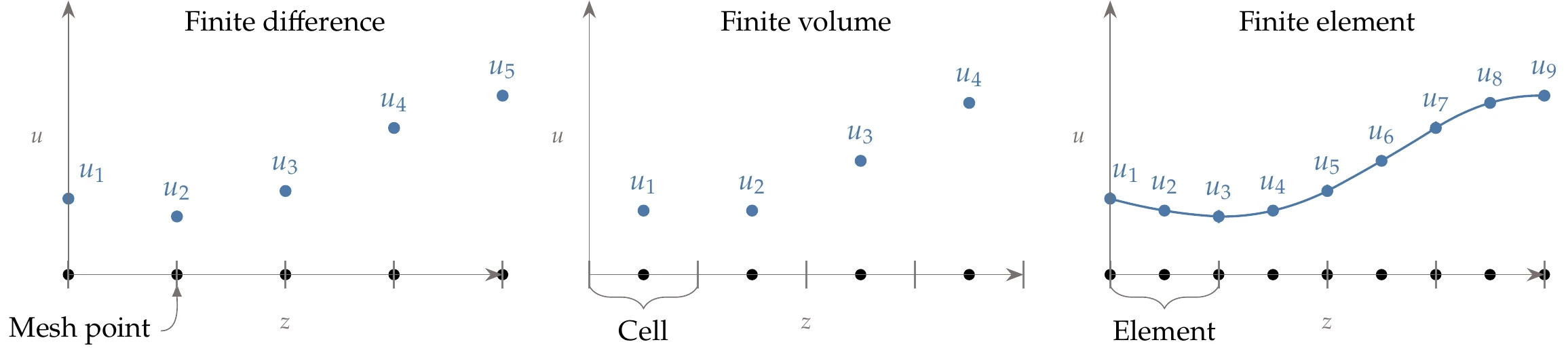
Figure 3.6:Discretization methods in one spatial dimension.

With any of these discretization methods, the final result is a set of algebraic equations that we can write as $r(u)=0$ and solve for the state variables $u$ . This is a potentially large set of equations depending on the domain and discretization (e.g., it is common to have millions of equations in three-dimensional computational fluid dynamics problems). The number of state variables of the discretized model is equal to the number of equations for a complete and well-defined model. In the most general case, the set of equations could be implicit and nonlinear.

When a problem involves both space and time, the prevailing approach is to decouple the discretization in space from the discretization in time—called the method of lines (see Figure 3.7). The discretization in space is performed first, yielding an ODE in time. The time derivative can then be approximated as a finite difference, leading to a time-integration scheme.

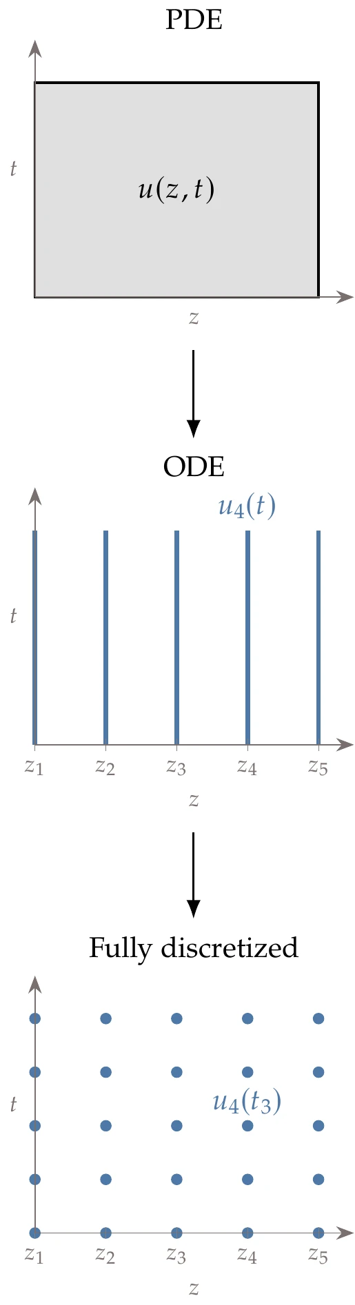
Figure 3.7:PDEs in space and time are often discretized in space first to yield an ODE in time.

The discretization process usually yields implicit algebraic equations that require a solver to obtain the solution. However, discretization in some cases yields explicit equations, in which case a solver is not required.

3.5 Numerical Errors¶

Numerical errors (or computation errors) can be categorized into three main types: roundoff errors, truncation errors, and errors due to coding. Numerical errors are involved with each of the modeling steps between the mathematical model and the states (see Figure 3.1). The error involved in the discretization step is a type of truncation error. The errors introduced in the coding step are not usually discussed as numerical errors, but we include them here because they are a likely source of error in practice. The errors in the computation step involve both roundoff and truncation errors. The following subsections describe each of these error sources.

An absolute error is the magnitude of the difference between the exact value ( $x^*$ ) and the computed value ( $x$ ), which we can write as $|x-x^*|$ . The relative error is a more intrinsic error measure and is defined as

\varepsilon = \frac{|x-x^*|}{|x^*|} \, .

(3.3)

This is the more useful error measure in most cases. When the exact value $x^*$ is close to zero, however, this definition breaks down. To address this, we avoid the division by zero by using

\varepsilon = \frac{|x-x^*|}{1 + |x^*|} \, .

(3.4)

This error metric combines the properties of absolute and relative errors. When $|x^*| \gg 1$ , this metric is similar to the relative error, but when $|x^*| \ll 1$ , it becomes similar to the absolute error.

3.5.1 Roundoff Errors¶

Roundoff errors stem from the fact that a computer cannot represent all real numbers with exact precision. Errors in the representation of each number lead to errors in each arithmetic operation, which in turn might accumulate throughout a program.

There is an infinite number of real numbers, but not all numbers can be represented in a computer. When a number cannot be represented exactly, it is rounded. In addition, a number might be too small or too large to be represented.

Computers use bits to represent numbers, where each bit is either 0 or 1. Most computers use the Institute of Electrical and Electronics Engineers (IEEE) standard for representing numbers and performing finite-precision arithmetic. A typical representation uses 32 bits for integers and 64 bits for real numbers.

Basic operations that only involve integers and whose result is an integer do not incur numerical errors. However, there is a limit on the range of integers that can be represented. When using 32-bit integers, 1 bit is used for the sign, and the remaining 31 bits can be used for the digits, which results in a range from $-2^{31}=-2,147,483,648$ to $2^{31}-1 = 2,147,483,647$ . Any operation outside this range would result in integer overflow.^[1]Real numbers are represented using scientific notation in base 2:

x = \text{significand} \times 2^{\text{exponent}} \, .

(3.5)

The 64-bit representation is known as the double-precision floating-point format, where some digits store the significand and others store the exponent. The greatest positive and negative real numbers that can be represented using the IEEE double-precision representation are approximately 10³⁰⁸ and -10³⁰⁸. Operations that result in numbers outside this range result in overflow, which is a fatal error in most computers and interrupts the program execution.

There is also a limit on how close a number can come to zero, approximately 10^-324 when using double precision. Numbers smaller than this result in underflow. The computer sets such numbers to zero by default, and the program usually proceeds with no harmful consequences.

One important number to consider in roundoff error analysis is the machine precision, $\varepsilon_\mathcal{M}$ , which represents the precision of the computations. This is the smallest positive number $\varepsilon$ such that

1 + \varepsilon > 1

(3.6)

when calculated using a computer. This number is also known as machine zero. Typically, the double precision 64-bit representation uses 1 bit for the sign, 11 bits for the exponent, and 52 bits for the significand. Thus, when using double precision, $\varepsilon_\mathcal{M} = 2^{-52} \approx 2.2 \times 10^{-16}$ . A double-precision number has about 16 digits of precision, and a relative representation error of up to $\varepsilon_\mathcal{M}$ may occur.

When operating with numbers that contain errors, the result is subject to a propagated error. For multiplication and division, the relative propagated error is approximately the sum of the relative errors of the respective two operands.

For addition and subtraction, an error can occur even when the two operands are represented exactly. Before addition and subtraction, the computer must convert the two numbers to the same exponent. When adding numbers with different exponents, several digits from the small number vanish (see Figure 3.8). If the difference in the two exponents is greater than the magnitude of the exponent of $\varepsilon_\mathcal{M}$ , the small number vanishes completely—a consequence of Equation 3.6. The relative error incurred in addition is still $\varepsilon_\mathcal{M}$ .

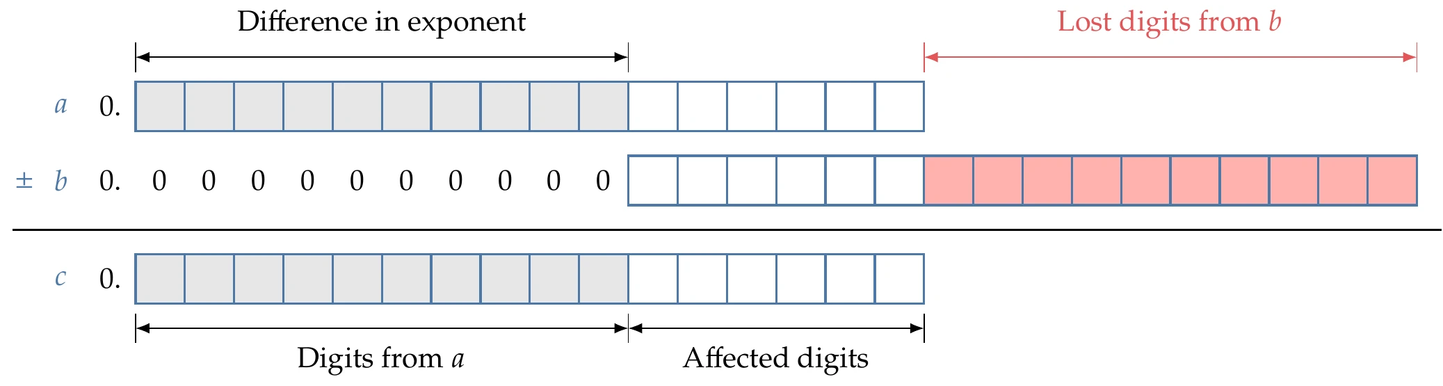
Figure 3.8:Adding or subtracting numbers of differing exponents results in a loss in the number of digits corresponding to the difference in the exponents. The gray boxes indicate digits that are identical between the two numbers.

On the other hand, subtraction can incur much greater relative errors when subtracting two numbers that have the same exponent and are close to each other. In this case, the digits that match between the two numbers cancel each other and reduce the number of significant digits. When the relative difference between two numbers is less than machine precision, all digits match, and the subtraction result is zero (see Figure 3.9). This is called subtractive cancellation and is a serious issue when approximating derivatives via finite differences (see Section 6.4).

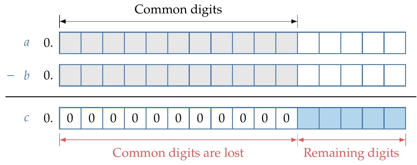
Figure 3.9:Subtracting two numbers that are close to each other results in a loss of the digits that match.

Sometimes, minor roundoff errors can propagate and result in much more significant errors. This can happen when a problem is ill-conditioned or when the algorithm used to solve the problem is unstable. In both cases, small changes in the inputs cause large changes in the output. Ill-conditioning is not a consequence of the finite-precision computations but is a characteristic of the model itself. Stability is a property of the algorithm used to solve the problem. When a problem is ill-conditioned, it is challenging to solve it in a stable way. When a problem is well conditioned, there is a stable algorithm to solve it.

Example 3.6 (Effect of roundoff error on function representation)

Figure 3.10:With double precision, the minimum of this quadratic function is in an interval much larger than machine zero.

Let us examine the function $f(x) = x^2 - 4x + 4$ near its minimum, at $x=2$ . If we use double precision and plot many points in a small interval, we can see that the function exhibits the step pattern shown in Figure 3.10. The numerical minimum of this function is anywhere in the interval around $x=2$ where the numerical value is zero. This interval is much larger than the machine precision ( $\varepsilon_\mathcal{M} = 2.2 \times 10^{-16}$ ). An additional error is incurred in the function computation around $x=2$ as a result of subtractive cancellation. This illustrates the fact that all functions are discontinuous when using finite-precision arithmetic.

3.5.2 Truncation Errors¶

In the most general sense, truncation errors arise from performing a finite number of operations where an infinite number of operations would be required to get an exact result.^[2] Truncation errors would arise even if we could do the arithmetic with infinite precision.

When discretizing a mathematical model with partial derivatives as described in Section 3.4, these are approximated by truncated Taylor series expansions that ignore higher-order terms. When the model includes integrals, they are approximated as finite sums. In either case, a mesh of points where the relevant states and functions are evaluated is required. Discretization errors generally decrease as the spacing between the points decreases.

3.5.3 Iterative Solver Tolerance Error¶

Many methods for solving numerical models involve an iterative procedure that starts with a guess for the states $u$ and then improves that guess at each iteration until reaching a specified convergence tolerance. The convergence is usually measured by a norm of the residuals, $\|r(u)\|$ , which we want to drive to zero. Iterative linear solvers and Newton-type solvers are examples of iterative methods (see Section 3.6).

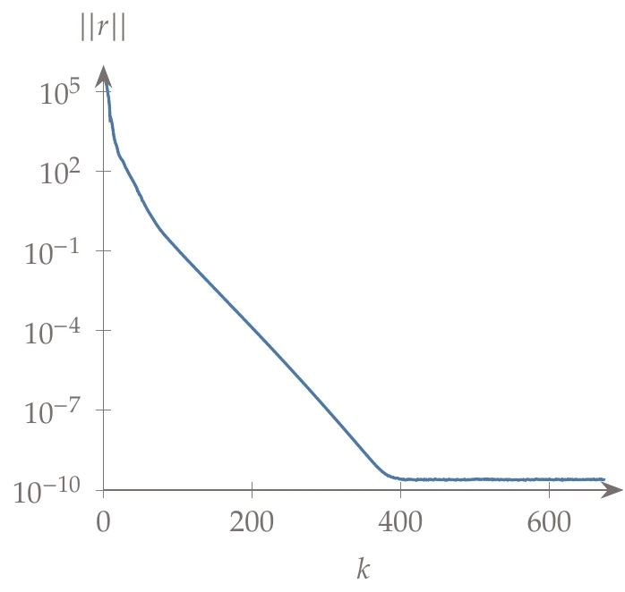
Figure 3.11:Norm of residuals versus the number of iterations for an iterative solver.

A typical convergence history for an iterative solver is shown in Figure 3.11. The norm of the residuals decreases gradually until a limit is reached (near 10^-10 in this case). This limit represents the lowest error achieved with the iterative solver and is determined by other sources of error, such as roundoff and truncation errors. If we terminate before reaching the limit (either by setting a convergence tolerance to a value higher than 10^-10 or setting an iteration limit to lower than 400 iterations), we incur an additional error. However, it might be desirable to trade off a less precise solution for a lower computational effort.

Tip 3.2: Find the level of the numerical noise in your model

It is crucial to know the error level in your model because this limits the type of optimizer you can use and how well you can optimize. In Example 3.6, we saw that if we plot a function at a small enough scale, we can see discrete steps in the function due to roundoff errors. When accumulating all sources of error in a more elaborate model (roundoff, truncation, and iterative), we no longer have a neat step pattern. Instead, we get numerical noise, as shown in Figure 3.12. The noise level can be estimated by the amplitude of the oscillations and gives us the order of magnitude of the total numerical error.

Figure 3.12:To find the level of numerical noise of a function of interest with respect to an input parameter (left), we magnify both axes by several orders of magnitude and evaluate the function at points that are closely spaced (right).

3.5.4 Programming Errors¶

Most of the literature on numerical methods is too optimistic and does not explicitly discuss programming errors, commonly known as bugs. Most programmers, especially beginners, underestimate the likelihood that their code has bugs.

It is helpful to adopt sound programming practices, such as writing clear, modular code. Clear code has consistent formatting, meaningful naming of variable functions, and helpful comments. Modular code reuses and generalizes functions as much as possible and avoids copying and pasting sections of code.2 Modular code allows for more flexible usage. Breaking up programs into smaller functions with well-defined inputs and outputs makes debugging much more manageable.^[3]There are different types of bugs relevant to numerical models: generic programming errors, incorrect memory handling, and algorithmic or logical errors. Programming errors are the most frequent and include typos, type errors, copy-and-paste errors, faulty initializations, missing logic, and default values.

In theory, careful programming and code inspection can avoid these errors, but you must always test your code in practice. This testing involves comparing your result with a case where you know the solution—the reference result. You should start with the simplest representative problem and then build up from that. Interactive debuggers are helpful because let you step through the code and check intermediate variable values.

Tip 3.3: Debugging is a skill that takes practice

The overall attitude toward programming should be that all code has bugs until it is verified through testing. Programmers who are skilled at debugging are not necessarily any better at spotting errors by reading code or by stepping through a debugger than average programmers. Instead, effective programmers use a systematic approach to narrow down where the problem is occurring.

Beginners often try to debug by running the entire program. Even experienced programmers have a hard time debugging at that level. One primary strategy discussed in this section is to write modular code. It is much easier to test and debug small functions. Reliable complex programs are built up through a series of well-tested modular functions. Sometimes we need to simplify or break up functions even further to narrow down the problem. We might need to streamline and remove pieces, make sure a simple case works, then slowly rebuild the complexity.

You should also become comfortable reading and understanding the error messages and stack traces produced by the program. These messages seem obscure at first, but through practice and researching what the error messages mean, they become valuable information sources.

Of course, you should carefully reread the code, looking for errors, but reading through it again and again is unlikely to yield new insights. Instead, it can be helpful to step away from the code and hypothesize the most likely ways the function could fail. You can then test and eliminate hypotheses to narrow down the problem.

Memory handling issues are much less frequent than programming errors, but they are usually more challenging to track.

These issues include memory leaks (a failure to free unused memory), incorrect use of memory management, buffer overruns (e.g., array bound violations), and reading uninitialized memory. Memory issues are challenging to track because they can result in strange behavior in parts of the code that are far from the source of the error. In addition, they might manifest themselves in specific conditions that are hard to reproduce consistently. Memory debuggers are essential tools for addressing memory issues. They perform detailed bookkeeping of all allocation, deallocation, and memory access to detect and locate any irregularities.^[4]

Whereas programming errors are due to a mismatch between the programmer’s intent and what is coded, the root cause of algorithmic or logical errors is in the programmer’s intent itself. Again, testing is the key to finding these errors, but you must be sure that the reference result is correct.

Running the analysis within an optimization loop can reveal bugs that do not manifest themselves in a single analysis. Therefore, you should only run an optimization test case after you have tested the analysis code in isolation.

As previously mentioned, there is a higher incentive to reduce the computational cost of an analysis when it runs in an optimization loop because it will run many times. When you first write your code, you should prioritize clarity and correctness as opposed to speed. Once the code is verified through testing, you should identify any bottlenecks using a performance profiling tool. Memory performance issues can also arise from running the analysis in an optimization loop instead of running a single case. In addition to running a memory debugger, you can also run a memory profiling tool to identify opportunities to reduce memory usage.

3.6 Overview of Solvers¶

There are several methods available for solving the discretized governing equations (Equation 3.1). We want to solve the governing equations for a fixed set of design variables, so $x$ will not appear in the solution algorithms. Our objective is to find the state variables $u$ such that $r(u)=0$ .

This is not a book about solvers, but it is essential to understand the characteristics of these solvers because they affect the cost and precision of the function evaluations in the overall optimization process. Thus, we provide an overview and some of the most relevant details in this section.^[5] In addition, the solution of coupled systems builds on these solvers, as we will see in Section 13.2.

Finally, some of the optimization algorithms detailed in later chapters use these solvers.

There are two main types of solvers, depending on whether the equations to be solved are linear or nonlinear (Figure 3.13). Linear solution methods solve systems of the form $r(u)= A u - b = 0$ , where the matrix $A$ and vector $b$ are not dependent on $u$ . Nonlinear methods can handle any algebraic system of equations that can be written as $r(u) = 0$ .

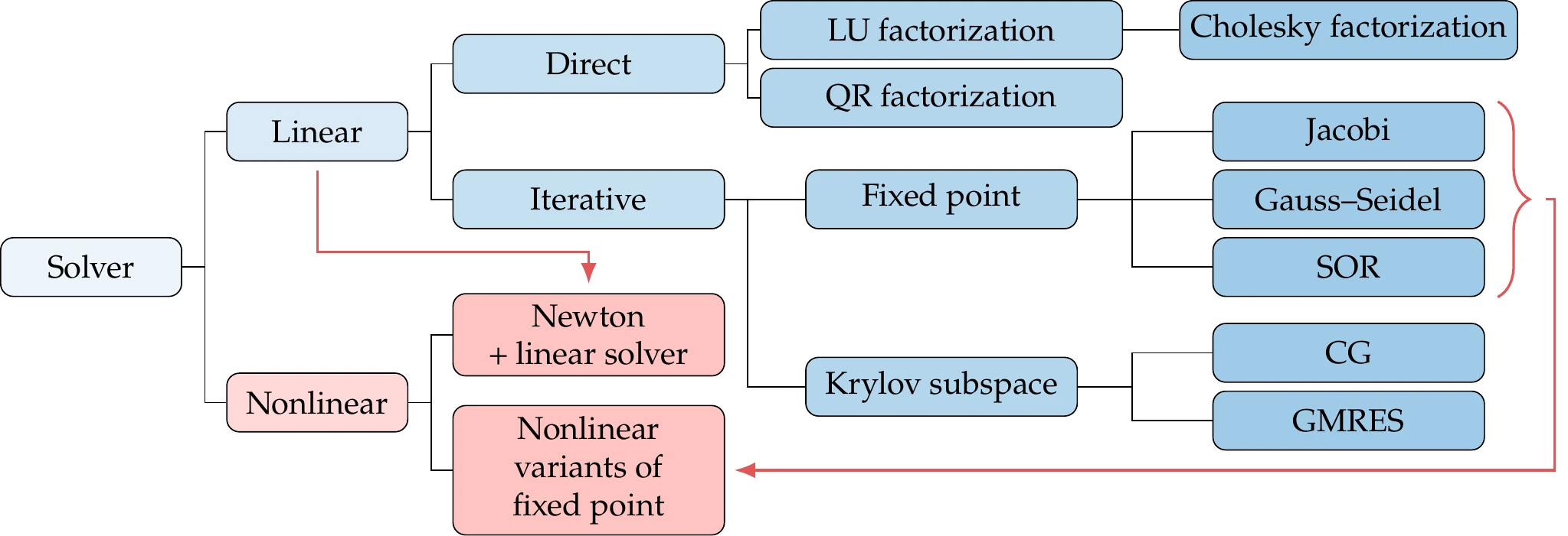
Figure 3.13:Overview of solution methods for linear and nonlinear systems.

Linear systems can be solved directly or iteratively. Direct methods are based on the concept of Gaussian elimination, which can be expressed in matrix form as a factorization into lower and upper triangular matrices that are easier to solve (LU factorization). Cholesky factorization is a more efficient variant of LU factorization that applies only to symmetric positive-definite matrices.

Whereas direct solvers obtain the solution $u$ at the end of a process, iterative solvers start with a guess for $u$ and successively improve it with each iteration, as illustrated in Figure 3.14.

Iterative methods can be fixed-point iterations, such as Jacobi, Gauss–Seidel, and successive over-relaxation (SOR), or Krylov subspace methods. Krylov subspace methods include the conjugate gradient (CG) and generalized minimum residual (GMRES) methods.^[6]

Direct solvers are well established and are included in the standard libraries for most programming languages. Iterative solvers are less widespread in standard libraries, but they are becoming more commonplace. describes linear solvers in more detail.

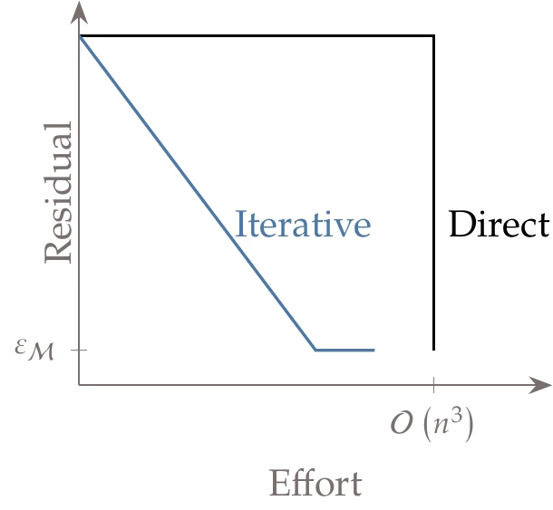
Figure 3.14:Whereas direct methods only yield the solution at the end of the process, iterative methods produce approximate intermediate results.

Direct methods are the right choice for many problems because they are generally robust. Also, the solution is guaranteed for a fixed number of operations, $\mathcal{O}(n^3)$ in this case.

However, for large systems where $A$ is sparse, the cost of direct methods can become prohibitive, whereas iterative methods remain viable. Iterative methods have other advantages, such as being able to trade between computational cost and precision. They can also be restarted from a good guess (see Iterative Methods).

When it comes to nonlinear solvers, the most efficient methods are based on Newton’s method, which we explain later in this chapter (Section 3.8). Newton’s method solves a sequence of problems that are linearizations of the nonlinear problem about the current iterate. The linear problem at each Newton iteration can be solved using any linear solver, as indicated by the incoming arrow in Figure 3.13.

Although efficient, Newton’s method is not robust in that it does not always converge. Therefore, it requires modifications so that it can converge reliably.

Finally, it is possible to adapt linear fixed-point iteration methods to solve nonlinear equations as well. However, unlike the linear case, it might not be possible to derive explicit expressions for the iterations in the nonlinear case. For this reason, fixed-point iteration methods are often not the best choice for solving a system of nonlinear equations.

However, as we will see in Section 13.2.5, these methods are useful for solving systems of coupled nonlinear equations.

For time-dependent problems, we require a way to solve for the time history of the states, $u(t)$ . As mentioned in Section 3.3, the most popular approach is to decouple the temporal discretization from the spatial one. By discretizing a PDE in space first, this method formulates an ODE in time of the following form:

\frac{\mathrm{d} u}{\mathrm{d} t} = -r(u,t) \, ,

(3.7)

which is called the semi-discrete form. A time-integration scheme is then used to solve for the time history. The integration scheme can be either explicit or implicit, depending on whether it involves evaluating explicit expressions or solving implicit equations.

If a system under a certain condition has a steady state, these techniques can be used to solve the steady state ( $\mathrm{d} u / \mathrm{d} t = 0$ ).

3.7 Rate of Convergence¶

Iterative solvers compute a sequence of approximate solutions that hopefully converge to the exact solution. When characterizing convergence, we need to first establish if the algorithm converges and, if so, how fast it converges. The first characteristic relates to the stability of the algorithm. Here, we focus on the second characteristic quantified through the rate of convergence.

The cost of iterative algorithms is often measured by counting the number of iterations required to achieve the solution. Iterative algorithms often require an infinite number of iterations to converge to the exact solution. In practice, we want to converge to an approximate solution close enough to the exact one. Determining the rate of convergence arises from the need to quantify how fast the approximate solution is approaching the exact one.

In the following, we assume that we have a sequence of points, $x_0, x_1, \ldots, x_k, \ldots$ , that represent approximate solutions in the form of vectors in any dimension and converge to a solution $x^*$ . Then,

\lim_{k \rightarrow \infty} \|x_k - x^*\| = 0 \, ,

(3.8)

which means that the norm of the error tends to zero as the number of iterations tends to infinity.

The rate of convergence of a sequence is of order $p$ with asymptotic error constant $\gamma$ when $p$ is the largest number that satisfies^[7]

0 \le \lim_{k \rightarrow \infty} \frac{\|x_{k+1} - x^*\|}{\|x_k - x^*\|^p} = \gamma < \infty \, .

(3.9)

Asymptotic here refers to the fact that this is the behavior in the limit, when we are close to the solution. There is no guarantee that the initial and intermediate iterations satisfy this condition.

To avoid dealing with limits, let us consider the condition expressed in Equation 3.9 at all iterations. We can relate the error from one iteration to the next by

\|x_{k+1} - x^*\| = \gamma_k \|x_k - x^*\|^p \, .

(3.10)

When $p=1$ , we have linear order of convergence; when $p=2$ , we have quadratic order of convergence. Quadratic convergence is a highly valued characteristic for an iterative algorithm, and in practice, orders of convergence greater than $p=2$ are usually not worthwhile to consider.

When we have linear convergence, then

\|x_{k+1} - x^*\| = \gamma_k \|x_k - x^*\| \, ,

(3.11)

where $\gamma_k$ converges to a constant but varies from iteration to iteration. In this case, the convergence is highly dependent on the value of the asymptotic error constant $\gamma$ . If $\gamma_k > 1$ , then the sequence diverges—a situation to be avoided. If $0 < \gamma_k < 1$ for every $k$ , then the norm of the error decreases by a constant factor for every iteration. Suppose that $\gamma = 0.1$ for all iterations. Starting with an initial error norm of 0.1, we get the sequence

10^{-1}, 10^{-2}, 10^{-3}, 10^{-4}, 10^{-5}, 10^{-6}, 10^{-7}, \ldots \, .

(3.12)

Thus, after six iterations, we get six-digit precision. Now suppose that $\gamma = 0.9$ . Then we would have

\begin{gather} 10^{-1}, 9.0 \times 10^{-2}, 8.1 \times 10^{-2}, 7.3 \times 10^{-2}, 6.6 \times 10^{-2}, \\ 5.9 \times 10^{-2}, 5.3 \times 10^{-2}, \ldots \, . \end{gather}

(3.13)

This corresponds to only one-digit precision after six iterations. It would take 131 iterations to achieve six-digit precision.

When we have quadratic convergence, then

\|x_{k+1} - x^*\| = \gamma_k \|x_k - x^*\|^2 \, .

(3.14)

If $\gamma =1$ , then the error norm sequence with a starting error norm of 0.1 would be

10^{-1}, 10^{-2}, 10^{-4}, 10^{-8}, \ldots \, .

(3.15)

This yields more than six digits of precision in just three iterations! In this case, the number of correct digits doubles at every iteration. When $\gamma > 1$ , the convergence will not be as fast, but the series will still converge.

If $p \ge 1$ and $\lim_{k \rightarrow \infty}\gamma_k = 0$ , we have superlinear convergence, which includes quadratic and higher rates of convergence. There is a special case of superlinear convergence that is relevant for optimization algorithms, which is when $p=1$ and $\gamma \rightarrow 0$ . This case is desirable because in practice, it behaves similarly to quadratic convergence and can be achieved by gradient-based algorithms that use first derivatives (as opposed to second derivatives). In this case, we can write

\|x_{k+1} - x^*\| = \gamma_k \|x_k - x^*\| \, ,

(3.16)

where $\lim_{k \rightarrow \infty} \gamma_k = 0$ . Now we need to consider a sequence of values for $\gamma$ that tends to zero. For example, if $\gamma_k = 1/(k+1)$ , starting with an error norm of 0.1, we get

\begin{gather} 10^{-1}, 5 \times 10^{-1}, 1.7 \times 10^{-1}, 4.2 \times 10^{-2}, 8.3 \times 10^{-4}, \\ 1.4 \times 10^{-4}, 2.0 \times 10^{-5}, \ldots \, . \end{gather}

(3.17)

Thus, we achieve four-digit precision after six iterations. This special case of superlinear convergence is not quite as good as quadratic convergence, but it is much better than either of the previous linear convergence examples.

We plot these sequences in Figure 3.15. Because the points are just scalars and the exact solution is zero, the error norm is just $x_k$ . The first plot uses a linear scale, so we cannot see any differences beyond two digits. To examine the differences more carefully, we need to use a logarithmic axis for the sequence values, as shown in the plot on the right. In this scale, each decrease in order of magnitude represents one more digit of precision.

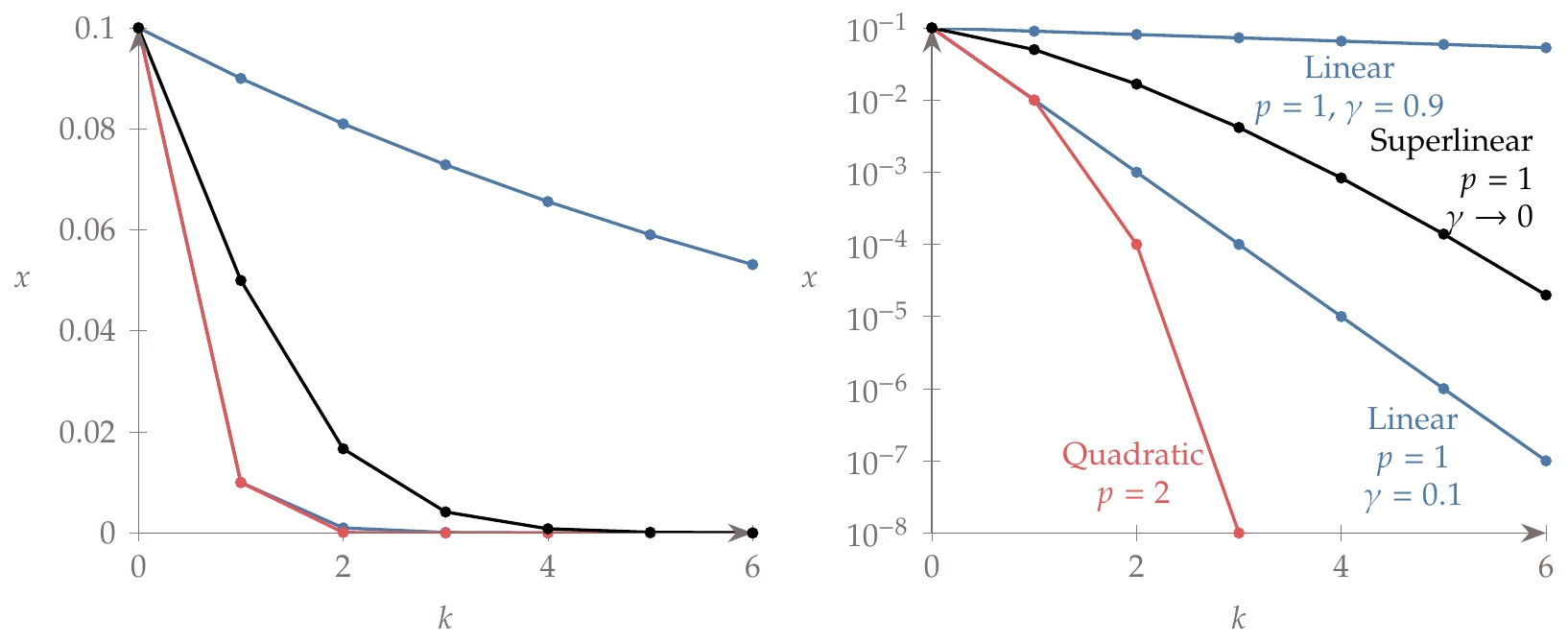
Figure 3.15:Sample sequences for linear, superlinear, and quadratic cases plotted on a linear scale (left) and a logarithmic scale (right).

The linear convergence sequences show up as straight lines in Figure 3.15 (right), but the slope of the lines varies widely, depending on the value of the asymptotic error constant. Quadratic convergence exhibits an increasing slope, reflecting the doubling of digits for each iteration. The superlinear sequence exhibits poorer convergence than the best linear one, but we can see that the slope of the superlinear curve is increasing, which means that for a large enough $k$ , it will converge at a higher rate than the linear one.

When solving numerical models iteratively, we can monitor the norm of the residual. Because we know that the residuals should be zero for an exact solution, we have

\|r_{k+1}\| = \gamma_k \|r_k\|^p \, .

(3.18)

If we monitor another quantity, we do not usually know the exact solution. In these cases, we can use the ratio of the step lengths of each iteration:

\frac{\|x_{k+1} - x^*\|}{\|x_k - x^*\|} \approx \frac{\|x_{k+1} - x_k\|}{\|x_k - x_{k-1}\|} \, .

(3.19)

The order of convergence can be estimated numerically with the values of the last available four iterates using

p \approx \dfrac{ \log_{10} \frac{ \|x_{k+1} - x_k\|} { \|x_k - x_{k-1}\|} } { \log_{10} \dfrac{ \|x_k - x_{k-1}\|} { \|x_{k-1} - x_{k-2}\|} } \, .

(3.20)

Finally, we can also monitor any quantity (function values, state variables, or design variables) by normalizing the step length in the same way as Equation 3.4,

\frac{\|x_{k+1} - x_k\|}{1 + \|x_k\|} \, .

(3.21)

3.8 Newton-Based Solvers¶

As mentioned in Section 3.6, Newton’s method is the basis for many nonlinear equation solvers. Newton’s method is also at the core of the most efficient gradient-based optimization algorithms, so we explain it here in more detail. We start with the single-variable case for simplicity and then generalize it to the $n$ -dimensional case.

We want to find $u^*$ such that $r(u^*)=0$ , where, for now, $r$ and $u$ are scalars. Newton’s method for root finding estimates a solution at each iteration $k$ by approximating $r \left(u_k \right)$ to be a linear function. The linearization is done by taking a Taylor series of $r$ about $u_k$ and truncating it to obtain the approximation

r \left( u_k + \Delta u \right) \approx r \left(u_k \right) + \Delta u r^\prime \left( u_k \right) \, ,

(3.22)

where $r^\prime = \mathrm{d} r / \mathrm{d} u$ . For conciseness, we define $r_k = r \left(u_k \right)$ . Now we can find the step $\Delta u$ that makes this approximate residual zero,

r_k + \Delta u {r^\prime_k} = 0 \quad \Rightarrow \quad \Delta u = - \frac{r_k}{{r^\prime_k}} \, ,

(3.23)

where we need to assume that $r^\prime_k \neq 0$ .

Thus, the update for each step in Newton’s algorithm is

u_{k+1} = u_k - \frac{r_k}{r^\prime_k} \, .

(3.24)

If $r^\prime_k = 0$ , the algorithm will not converge because it yields a step to infinity. Small enough values of $r^\prime_k$ also cause an issue with large steps, but the algorithm might still converge.

One useful modification of Newton’s method is to replace the derivative with a forward finite-difference approximation (see Section 6.4) based on the residual values of the current and last iterations,

r^\prime_k \approx \frac{r_{k+1} - r_k}{u_{k+1} - u_k} \, .

(3.25)

Then, the update is given by

u_{k+1} = u_k - {r_k} \left(\frac{u_{k+1} - u_k} {r_{k+1} - r_k}\right) \, .

(3.26)

This is the secant method, which is useful when the derivative is not available. The convergence rate is not quadratic like Newton’s method, but it is superlinear.

Example 3.7 (Newton’s method and the secant method for a single variable)

Suppose we want to solve the equation $r(u) = 2 u^3 + 4u^2 + u - 2 = 0$ . Because $r^\prime(u) = 6 u^2 + 8 u + 1$ , the Newton iteration is

u_{k+1} = u_k - \frac{2 u_{k}^3 + 4u_{k}^2 + u_k - 2}{6 u_{k}^2 + 8 u_k + 1} \, .

When we start with the guess $u_0=1.5$ (left plot in Figure 3.16), the iterations are well behaved, and the method converges quadratically. We can see the geometric interpretation of Newton’s method: For each iteration, it takes the tangent to the curve and finds the intersection with $r=0$ .

Figure 3.16:Newton iterations starting from different starting points.

When we start with $u_0=-0.5$ (right plot in Figure 3.16), the first step goes in the wrong direction but recovers in the second iteration. The third iteration is close to the point with the zero derivative and takes a large step. In this case, the iterations recover and then converge normally. However, we can easily envision a case where an iteration is much closer to the point with the zero derivative, causing an arbitrarily long step.

Figure 3.17:Secant method applied to a one-dimensional function.

We can also use the secant method (Equation 3.26) for this problem, which gives the following update:

u_{k+1} = u_k - \frac{ \left( 2 u_{k}^3 + 4u_{k}^2 + u_k - 2 \right) \left( u_{k+1} - u_k \right)} {2 u_{k+1}^3 + 4u_{k+1}^2 + u_{k+1} - 2 u_{k}^3 - 4u_{k}^2 - u_k} \, .

The iterations for the secant method are shown in Figure 3.17, where we can see the successive secant lines replacing the exact tangent lines used in Newton’s method.

Newton’s method converges quadratically as it approaches the solution with a convergence constant of

\gamma = \left| \frac{r^{\prime\prime}(u^*)}{2 r^\prime (u^*)} \right| \, .

(3.27)

This means that if the derivative is close to zero or the curvature tends to a large number at the solution, Newton’s method will not converge as well or not at all.

Now we consider the general case where we have $n$ nonlinear equations of $n$ unknowns, expressed as $r(u)=0$ . Similar to the single-variable case, we derive the Newton step from a truncated Taylor series. However, the Taylor series needs to be multidimensional in both the independent variable and the function. Consider first the multidimensionality of the independent variable, $u$ , for a component of the residuals, $r_i(u)$ . The first two terms of the Taylor series about $u_k$ for a step $\Delta u$ (which is now a vector with arbitrary direction and magnitude) are

r_i\left(u_k+ \Delta u \right) \approx r_i\left(u_k \right) + \sum_{j=1}^n \Delta u_j \frac{\partial {r_i}}{\partial {u_j}}\Bigr\rvert_{u = u_k} \, .

(3.28)

Because we have $n$ residuals, $i=1,\ldots,n$ , we can write the second term in matrix form as $J \Delta u$ , where $J$ is an $(n \times n)$ square matrix whose elements are

J_{ij} = \frac{\partial {r_i}}{\partial {u_j}}\, .

(3.29)

This matrix is called the Jacobian.

Similar to the single-variable case, we want to find the step that makes the two terms zero, which yields the linear system

J_k \Delta u_k = -r_k \, .

(3.30)

After solving this linear system, we can update the solution to

u_{k+1} = u_k + \Delta u_k \, .

(3.31)

Thus, Newton’s method involves solving a sequence of linear systems given by Equation 3.30. The linear system can be solved using any of the linear solvers mentioned in Section 3.6.

One popular option for solving the Newton step is the Krylov method, which results in the Newton–Krylov method for solving nonlinear systems. Because the Krylov method only requires matrix-vector products of the form $J v$ , we can avoid computing and storing the Jacobian by computing this product directly (using finite differences or other methods from Chapter 6). In Section 4.4.3 we adapt Newton’s method to perform function minimization instead of solving nonlinear equations.

The multivariable version of Newton’s method is subject to the same issues we uncovered for the single-variable case: it only converges if the starting point is within a specific region, and it can be subject to ill-conditioning. To increase the likelihood of convergence from any starting point, Newton’s method requires a globalization strategy (see Section 4.2). The ill-conditioning issue has to do with the linear system (Equation 3.30) and can be quantified by the condition number of the Jacobian matrix. Ill-conditioning can be addressed by scaling and preconditioning.

There is an analog of the secant method for $n$ dimensions, which is called Broyden’s method. This method is much more involved than its one-dimensional counterpart because it needs to create an approximate Jacobian based on directional finite-difference derivatives. Broyden’s method is described in Section C.1 and is related to the quasi-Newton optimization methods of Section 4.4.4.

Example 3.8 (Newton’s method applied to two nonlinear equations)

Suppose we have the following nonlinear system of two equations:

u_2 = \frac{1}{u_1}, \quad u_2 = \sqrt{u_1} \, .

Figure 3.18:Newton iterations.

This corresponds to the two lines shown in Figure 3.18, where the solution is at their intersection, $u=(1,1)$ . (In this example, the two equations are explicit, and we could solve them by substitution, but they could have been implicit.)

To solve this using Newton’s method, we need to write these as residuals:

\begin{aligned} r_1 &= u_2 - \frac{1}{u_1} = 0 \\ r_2 &= u_2 - \sqrt{u_1} = 0 \, . \end{aligned}

The Jacobian can be derived analytically, and the Newton step is given by the linear system

\begin{bmatrix} \frac{1}{u_1^2} & 1 \\ -\frac{1}{2 \sqrt{u_1}} & 1 \end{bmatrix} \begin{bmatrix} \Delta u_1 \\ \Delta u_2 \end{bmatrix} = - \begin{bmatrix} u_2 - \frac{1}{u_1} \\ u_2 - \sqrt{u_1} \end{bmatrix} \, .

Starting from $u=(2,3)$ yields the iterations shown in the following table, with the quadratic convergence shown in Figure 3.19.

Figure 3.19:The norm of the residual exhibits quadratic convergence.

$u_1$	$u_2$	$\\|u-u^*\\|$	$\\|r\\|$
2.000000	3.000000	2.24	2.96
0.485281	0.878680	5.29e-1	1.20
0.760064	0.893846	2.62e-1	4.22e-1
0.952668	0.982278	5.05e-2	6.77e-2
0.998289	0.999417	1.81e-3	2.31e-3
0.999998	0.999999	2.32e-6	2.95e-6
1.000000	1.000000	3.82e-12	4.87e-12
1.000000	1.000000	0.0	0.0

3.9 Models and the Optimization Problem¶

When performing design optimization, we must compute the values of the objective and constraint functions in the optimization problem (Equation 1.4). Computing these functions usually requires solving a model for the given design $x$ at one or more specific conditions.^[8]The model often includes governing equations that define the state variables $u$ as an implicit function of $x$ . In other words, for a given $x$ , there is a $u$ that solves $r(u;x)=0$ , as illustrated in Figure 3.20. Here, the semicolon in $r(u; x)$ indicates that $x$ is fixed when the governing equations are solved for $u$ .

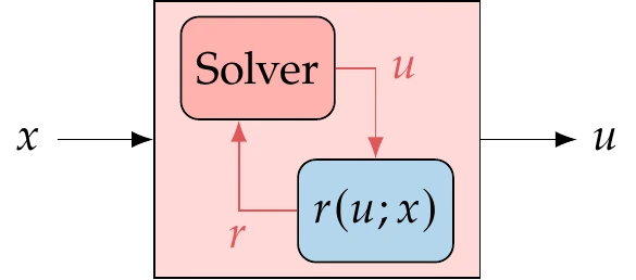
For a general model, the state variables u are implicit functions of the design variables x through the solution of the governing equations. — Figure 3.20:For a general model, the state variables $u$ are implicit functions of the design variables $x$ through the solution of the governing equations.

The objective and constraints are typically explicit functions of the state and design variables, as illustrated in Figure 3.21 (this is a more detailed version of Figure 1.14).

There is also an implicit dependence of the objective and constraint functions on $x$ through $u$ . Therefore, the objective and constraint functions are ultimately fully determined by the design variables. In design optimization applications, solving the governing equations is usually the most computationally intensive part of the overall optimization process.

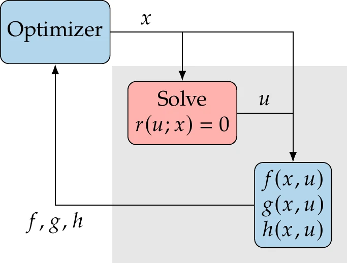
Computing the objective (f) and constraint functions (g,h) for a given set of design variables (x) usually involves the solution of a numerical model (r=0) by varying the state variables (u). — Figure 3.21:Computing the objective ( $f$ ) and constraint functions ( $g$ , $h$ ) for a given set of design variables ( $x$ ) usually involves the solution of a numerical model ( $r=0$ ) by varying the state variables ( $u$ ).

When we first introduced the general optimization problem (Equation 1.4), the governing equations were not included because they were assumed to be part of the computation of the objective and constraints for a given $x$ . However, we can include them in the problem statement for completeness as follows:

\begin{aligned} \text{minimize} &\quad f(x; u) \\ \text{by varying} &\quad x_i & i &= 1, \ldots, n_x \\ \text{subject to} & \quad g_j(x; u) \le 0 & j &= 1, \ldots, n_g \\ & \quad h_k(x; u) = 0 & k &= 1, \ldots, n_{h}\\ & \quad \underline{x}_i \le x_i \le \overline{x}_i & i &= 1, \ldots, n_x \\ \text{while solving} &\quad r_l(u; x) = 0 & l &= 1, \ldots, n_u \\ \text{by varying} &\quad u_l & l &= 1, \ldots, n_u \, . \end{aligned}

(3.32)

Here, “while solving” means that the governing equations are solved at each optimization iteration to find a valid $u$ for each value of $x$ . The semicolon in $f(x; u)$ indicates that $u$ is fixed while the optimizer determines the next value of $x$ .

Example 3.9 (Structural sizing optimization)

Recalling the truss problem of Example 3.2, suppose we want to minimize the mass of the structure ( $m$ ) by varying the cross-sectional areas of the truss members ( $a$ ), subject to stress constraints.

The structural mass is an explicit function that can be written as

m = \sum_{i=1}^{15} \rho a_i l_i,

where $\rho$ is the material density, $a_i$ is the cross-sectional area of each member $i$ , and $l_i$ is the member length. This function depends on the design variables directly and does not depend on the displacements.

We can write the optimization problem statement as follows:

\begin{aligned} \text{minimize} &\quad m(a) \\ \text{by varying} &\quad a_i \ge a_{\text{min}} & i = 1, \ldots, 15 \\ \text{subject to} & \quad |\sigma_j(a,u)| - \sigma_\text{max} \le 0 & j = 1, \ldots, 15 \\ \text{while solving} &\quad K u - q = 0 & (\text{system of 18 equations}) \\ \text{by varying} &\quad u_l & l = 1, \ldots, 18 \, . \end{aligned}

The governing equations are a linear set of equations whose solution determines the displacements ( $u$ ) of a given design ( $a$ ) for a load condition ( $q$ ). We mentioned previously that the objective and constraint functions are usually explicit functions of the state variables, design variables, or both. As we saw in Example 3.2, the mass is an explicit function of the cross-sectional areas. In this case, it does not even depend on the state variables. The constraint function is also explicit, but in this case, it is just a function of the state variables. This example illustrates a common situation where the solution of the state variables requires the solution of implicit equations (structural solver), whereas the constraints (stresses) and objective (weight) are explicit functions of the states and design variables.

From a mathematical perspective, the model governing equations $r(x,u)=0$ can be considered equality constraints in an optimization problem. Some specialized optimization approaches add these equations to the optimization problem and let the optimization algorithm solve both the governing equations and optimization simultaneously. This is called a full-space approach and is also known as simultaneous analysis and design (SAND) or one-shot optimization.

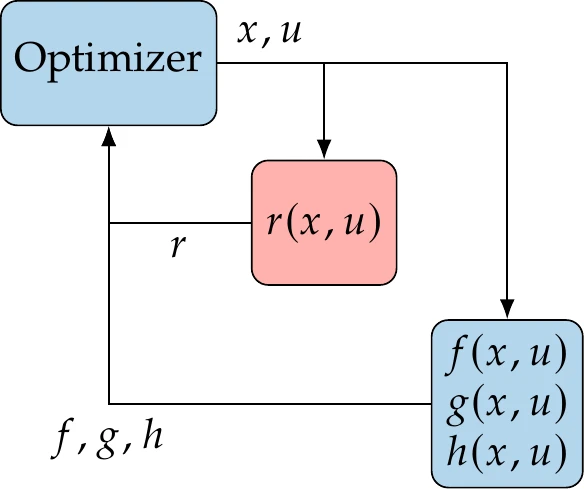
Figure 3.22:In the full-space approach, the governing equations are solved by the optimizer by varying the state variables.

The approach is illustrated in Figure 3.22 and stated as follows:

\begin{aligned} \text{minimize} &\quad f(x, u) \\ \text{by varying} &\quad x_i & i &= 1, \ldots, n_x \\ &\quad u_l & l &= 1, \ldots, n_u \\ \text{subject to} & \quad g_j(x,u) \le 0 & j &= 1, \ldots, n_g \\ & \quad h_k(x,u) = 0 & k &= 1, \ldots, n_{h}\\ & \quad \underline{x}_i \le x_i \le \overline{x}_i & i &= 1, \ldots, n_x \\ &\quad r_l(x,u) = 0 & l &= 1, \ldots, n_u \, . \end{aligned}

(3.33)

This approach is described in more detail in Section 13.4.3.

More generally, the optimization constraints and equations in a model are interchangeable. Suppose a set of equations in a model can be satisfied by varying a corresponding set of state variables. In that case, these equations and variables can be moved to the optimization problem statement as equality constraints and design variables, respectively.

Unless otherwise stated, we assume that the optimization model governing equations are solved by a dedicated solver for each optimization iteration, as stated in Equation 3.32.

Example 3.10 (Structural sizing optimization using a full-space approach)

To solve the structural sizing problem (Example 3.9) using a full-space approach, we forgo the linear solver by adding $u$ to the set of design variables and letting the optimizer enforce the governing equations. This results in the following problem:

\begin{aligned} \text{minimize} &\quad m(a) \\ \text{by varying} &\quad a_i \ge a_\text{min} & i = 1, \ldots, 15 \\ &\quad u_l & l = 1, \ldots, 18 \\ \text{subject to} & \quad |\sigma_j(a,u)| - \sigma_\text{max} \le 0 & j = 1, \ldots, 15 \\ &\quad K u - q = 0 & \text{(system of 18 equations)} \, . \end{aligned}

3.10 Summary¶

It is essential to understand the models that compute the objective and constraint functions because they directly affect the performance and effectiveness of the optimization process.

The modeling process introduces several types of numerical errors associated with each step of the process (discretization, programming, computation), limiting the achievable precision of the optimization. Knowing the level of numerical error is necessary to establish what precision can be achieved in the optimization. Understanding the types of errors involved helps us find ways to reduce those errors. Programming errors—“bugs”—are often underestimated; thorough testing is required to verify that the numerical model is coded correctly. A lack of understanding of a given model’s numerical errors is often the cause of a failure in optimization, especially when using gradient-based algorithms.

Modeling errors arise from discrepancies between the mathematical model and the actual physical system. Although they do not affect the optimization process’s performance and precision, modeling errors affect the accuracy and determine how valid the result is in the real world. Therefore, model validation and an understanding of modeling error are also critical.

In engineering design optimization problems, the models usually involve solving large sets of nonlinear implicit equations. The computational time required to solve these equations dominates the overall optimization time, and therefore, solver efficiency is crucial. Solver robustness is also vital because optimization often asks for designs that are very different from what a human designer would ask for, which tests the limits of the model and the solver.

We presented an overview of the various types of solvers available for linear and nonlinear equations. Newton-type methods are highly desirable for solving nonlinear equations because they exhibit second-order convergence. Because Newton-type methods involve solving a linear system at each iteration, a linear solver is always required. These solvers are also at the core of several of the optimization algorithms in later chapters.

Problems¶

Exercise 1

Answer true or false and justify your answer.

A model developed to perform well for analysis will always do well in a numerical optimization process.
Modeling errors have nothing to do with computations.
Explicit and implicit equations can always be written in residual form.
Subtractive cancellation is a type of roundoff error.
Programming errors can always be eliminated by carefully reading the code.
Quadratic convergence is only better than linear convergence if the asymptotic convergence error constant is less than or equal to one.
Logarithmic scales are desirable when plotting convergence because they show errors of all magnitudes.
Newton solvers always require a linear solver.
Some linear iterative solvers can be used to solve nonlinear problems.
Direct methods allow us to trade between computational cost and precision, whereas iterative methods do not.
Newton’s method requires the derivatives of all the state variables with respect to the residuals.
In the full-space optimization approach, the state variables become design variables, and the governing equations become constraints.

Exercise 6

Kepler’s equation, which we mentioned in Section 2.2, defines the relationship between a planet’s polar coordinates and the time elapsed from a given initial point and is stated as follows:

E - e \sin (E) = M ,

(3.36)

where $M$ is the mean anomaly (a parameterization of time), $E$ is the eccentric anomaly (a parameterization of polar angle), and $e$ is the eccentricity of the elliptical orbit.

Use Newton’s method to find $E$ when $e=0.7$ and $M=\pi/2$ .
Devise a fixed-point iteration to solve the same problem.
Compare the number of iterations and rate of convergence.
Exploration: Plot $E$ versus $M$ in the interval $[0, 2\pi]$ for $e=[0, 0.1, 0.5, 0.9]$ and interpret your results physically.

Footnotes¶

Some programming languages, such as Python, have arbitrary precision integers and are not subject to this issue, albeit with some performance trade-offs.
↩
Roundoff error, discussed in the previous section, is sometimes also referred to as truncation error because digits are truncated. However, we avoid this confusing naming and only use truncation error to refer to a truncation in the number of operations.
↩
The term debugging was used in engineering prior to computers, but Grace Hopper popularized this term in the programming context after a glitch in the Harvard Mark II computer was found to be caused by a moth.
↩
See 3 for more details on how to debug and profile code.
↩
4 provide a more detailed introduction to the numerical methods mentioned in this chapter.
↩
See 5 for more details on iterative methods in the context of large-scale numerical models.
↩
Some authors refer to $p$ as the rate of convergence. Here, we characterize the rate of convergence by two metrics: order and error constant.
↩
As previously mentioned, the process of solving a model is also known as the analysis or simulation.
↩

References¶

Box, G. E. P. (1976). Science and statistics. Journal of the American Statistical Association, 71(356), 791–799. 10.2307/2286841
Wilson, G., Aruliah, D. A., Brown, C. T., Hong, N. P. C., Davis, M., Guy, R. T., Haddock, S. H. D., Huff, K. D., Mitchell, I. M., Plumbley, M. D., Waugh, B., White, E. P., & Wilson, P. (2014). Best practices for scientific computing. PLoS Biology, 12(1), e1001745. 10.1371/journal.pbio.1001745
Grotker, T., Holtmann, U., Keding, H., & Wloka, M. (2012). The Developer’s Guide to Debugging (2nd ed.). Springer. https://www.google.ca/books/edition/The_Developer_s_Guide_to_Debugging/OlHMSAAACAAJ
Ascher, U. M., & Greif, C. (2011). A First Course in Numerical Methods. SIAM. https://www.google.ca/books/edition/A_First_Course_in_Numerical_Methods/eGDMSIqPYdYC
Saad, Y. (2003). Iterative Methods for Sparse Linear Systems (2nd ed.). SIAM. https://www.google.ca/books/edition/Iterative_Methods_for_Sparse_Linear_Syst/qtzmkzzqFmcC