2 A Short History of Optimization
This chapter provides helpful historical context for the methods discussed in this book. Nothing else in the book depends on familiarity with the material in this chapter, so it can be skipped. However, this history makes connections between the various topics that will enrich the big picture of optimization as you become familiar with the material in the rest of the book, so you might want to revisit this chapter.
Optimization has a long history that started with geometry problems solved by ancient Greek mathematicians. The invention of algebra and calculus opened the door to many more types of problems, and the advent of numerical computing increased the range of problems that could be solved in terms of type and scale.
2.1 The First Problems: Optimizing Length and Area
Ancient Greek and Egyptian mathematicians made numerous contributions to geometry, including solving optimization problems that involved length and area. They adopted a geometric approach to solving problems that are now more easily solved using calculus.
Archimedes of Syracuse (287–212 BCE) showed that of all possible spherical caps of a given surface area, hemispherical caps have the largest volume.
Euclid of Alexandria (325–265 BCE) showed that the shortest distance between a point and a line is the segment perpendicular to that line. He also proved that among rectangles of a given perimeter, the square has the largest area.
Geometric problems involving perimeter and area had practical value. The classic example of such practicality is Dido’s problem. According to the legend, Queen Dido, who had fled to Tunis, purchased from a local leader as much land as could be enclosed by an ox’s hide.
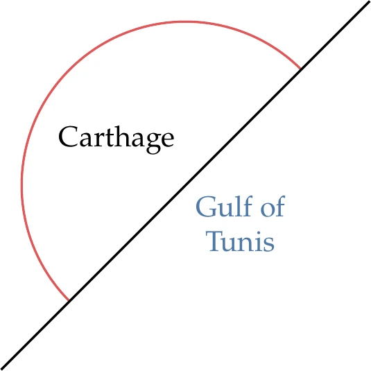
Figure 2.1:Queen Dido intuitively maximized the area for a given perimeter, thus acquiring enough land to found the city of Carthage.
The leader agreed because this seemed like a modest amount of land. To maximize her land area, Queen Dido had the hide cut into narrow strips to make the longest possible string. Then, she intuitively found the curve that maximized the area enclosed by the string: a semicircle with the diameter segment set along the sea coast (see Figure 2.1). As a result of the maximization, she acquired enough land to found the ancient city of Carthage. Later, Zenodorus (200–140 BCE) proved this optimal solution using geometrical arguments. A rigorous solution to this problem requires using calculus of variations, which was invented much later.
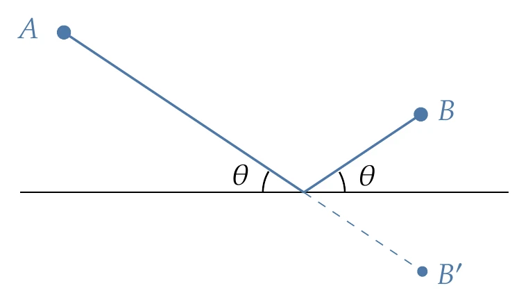
Figure 2.2:The law of reflection can be derived by minimizing the length of the light beam.
Geometric optimization problems are also applicable to the laws of physics. Hero of Alexandria (10–70 CE) derived the law of reflection by finding the shortest path for light reflecting from a mirror, which results in an angle of reflection equal to the angle of incidence (Figure 2.2).
2.2 Optimization Revolution: Derivatives and Calculus
The scientific revolution generated significant optimization developments in the seventeenth and eighteenth centuries that intertwined with other developments in mathematics and physics.
In the early seventeenth century, Johannes Kepler published a book in which he derived the optimal dimensions of a wine barrel.1 He became interested in this problem when he bought a barrel of wine, and the merchant charged him based on a diagonal length (see Figure 2.3). This outraged Kepler because he realized that the amount of wine could vary for the same diagonal length, depending on the barrel proportions.
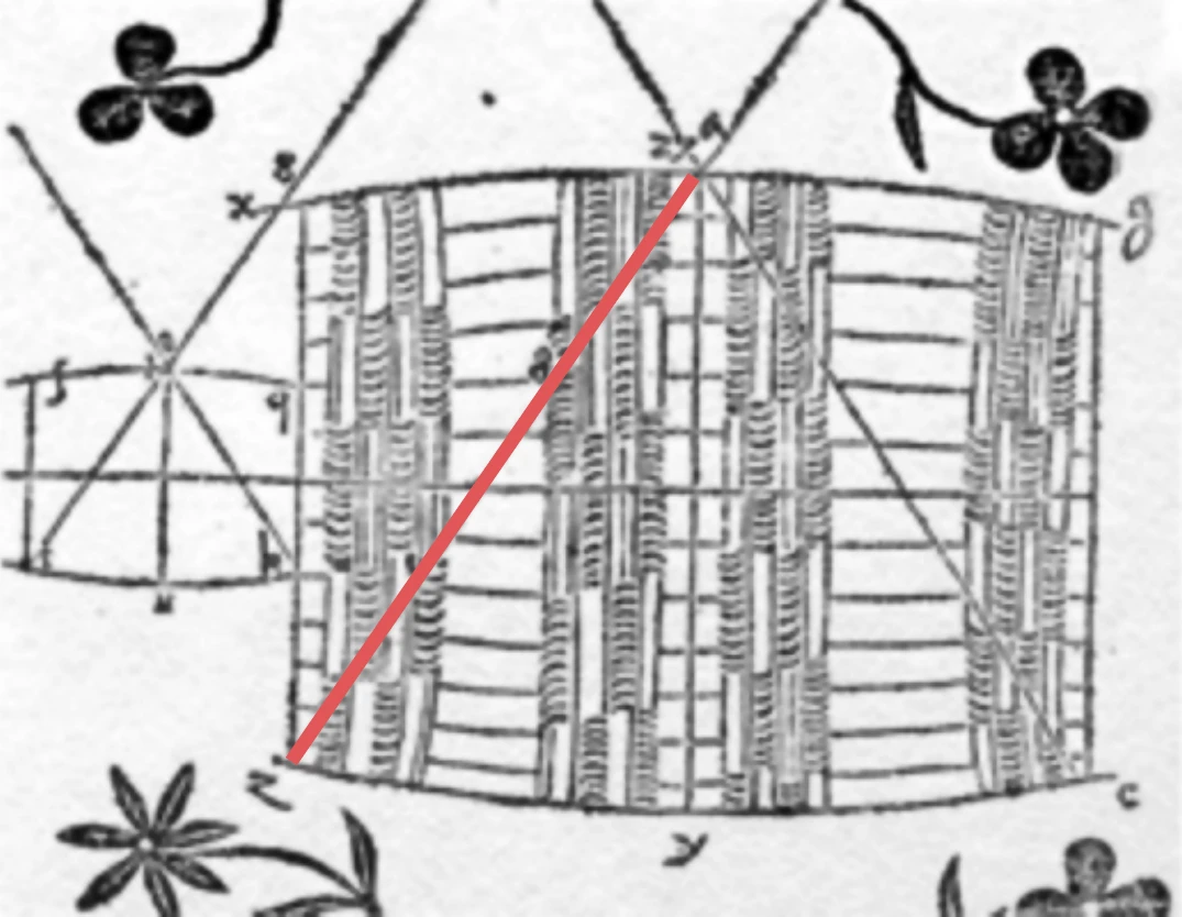
Figure 2.3:Wine barrels were measured by inserting a ruler in the tap hole until it hit the corner.
Incidentally, Kepler also formulated an optimization problem when looking for his second wife, seeking to maximize the likelihood of satisfaction. This “marriage problem” later became known as the “secretary problem”, which is an optimal-stopping problem that has since been solved using dynamic optimization (mentioned in Section 1.4.6 and discussed in Section 8.5).2
Willebrord Snell discovered the law of refraction in 1621, a formula that describes the relationship between the angles of incidence and refraction when light passes through a boundary between two different media, such as air, glass, or water. Whereas Hero minimized the length to derive the law of reflection, Snell minimized time. These laws were generalized by Fermat in the principle of least time (or Fermat’s principle), which states that a ray of light going from one point to another follows the path that takes the least time.
Pierre de Fermat derived Snell’s law by applying the principle of least time, and in the process, he devised a mathematical technique for finding maxima and minima using what amounted to derivatives (he missed the opportunity to generalize the notion of derivative, which came later in the development of calculus).3 Today, we learn about derivatives before learning about optimization, but Fermat did the reverse.
During this period, optimization was not yet considered an important area of mathematics, and contributions to optimization were scattered among other areas. Therefore, most mathematicians did not appreciate seminal contributions in optimization at the time.
In 1669, Isaac Newton wrote about a numerical technique to find the roots of polynomials by successively linearizing them, achieving quadratic convergence.
In 1687, he used this technique to find the roots of a nonpolynomial equation (Kepler’s equation),[1]but only after using polynomial expansions.
In 1690, Joseph Raphson improved on Newton’s method by keeping all the decimals in each linearization and making it a fully iterative scheme. The multivariable “Newton’s method” that is widely used today was actually introduced in 1740 by Thomas Simpson. He generalized the method by using the derivatives (which allowed for solving nonpolynomial equations without expansions) and by extending it to a system of two equations and two unknowns.[2]
In 1685, Newton studied a shape optimization problem where he sought the shape of a body of revolution that minimizes fluid drag and even mentioned a possible application to ship design. Although he used the wrong model for computing the drag, he correctly solved what amounted to a calculus of variations problem.
In 1696, Johann Bernoulli challenged other mathematicians to find the path of a body subject to gravity that minimizes the travel time between two points of different heights. This is now a classic calculus of variations problem called the brachistochrone problem (Figure 2.4). Bernoulli already had a solution that he kept secret. Five mathematicians respond with solutions: Newton, Jakob Bernoulli (Johann’s brother), Gottfried Wilhelm von Leibniz, Ehrenfried Walther von Tschirnhaus, and Guillaume de l’H^opital. Newton reportedly started working on the problem as soon as he received it and stayed up all night before sending the solution anonymously to Bernoulli the next day.
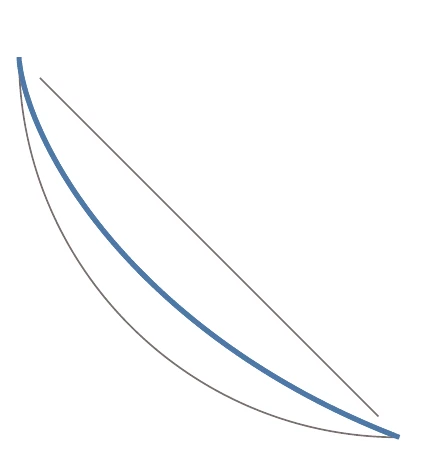
Figure 2.4:Suppose that you have a bead on a wire that goes from to . The brachistochrone curve is the shape of the wire that minimizes the time for the bead to slide between the two points under gravity alone. It is faster than a straight-line trajectory or a circular arc.
Starting in 1736, Leonhard Euler derived the general optimality conditions for solving calculus of variations problems, but the derivation included geometric arguments.
In 1755, Joseph-Louis Lagrange used a purely analytic approach to derive the same optimality conditions (he was 19 years old at the time!). Euler recognized Lagrange’s derivation, which uses variations of a function, as a superior approach and adopted it, calling it “calculus of variations”. This is a second-order partial differential equation that has become known as the Euler–Lagrange equation. Lagrange used this equation to develop a reformulation of classical mechanics in 1788, which became known as Lagrangian mechanics. When deriving the general equations of equilibrium for problems with constraints, Lagrange introduced the “method of the multipliers”.5 Lagrange multipliers eventually became a fundamental concept in constrained optimization (see Section 5.3).
In 1784, Gaspard Monge developed a geometric method to solve a transportation problem. Although the method was not entirely correct, it established combinatorial optimization, a branch of discrete optimization (Chapter 8).
2.3 The Birth of Optimization Algorithms
Several more theoretical contributions related to optimization occurred in the nineteenth century and the early twentieth century. However, it was not until the 1940s that optimization started to gain traction with the development of algorithms and their use in practical applications, thanks to the advent of computer hardware.
In 1805, Adrien-Marie Legendre described the method of least squares, which was used to predict asteroid orbits and for curve fitting. Friedrich Gauss published a rigorous mathematical foundation for the method of least squares and claimed he used it to predict the orbit of the asteroid Ceres in 1801. Legendre and Gauss engaged in a bitter dispute on who first developed the method.
In one of his 789 papers, Augustin-Louis Cauchy proposed the steepest-descent method for solving systems of nonlinear equations.6 He did not seem to put much thought into it and promised a “paper to follow” on the subject, which never happened. He proposed this method for solving systems of nonlinear equations, but it is directly applicable to unconstrained optimization (see Section 4.4.1).
In 1902, Gyula Farkas proved a theorem on the solvability of a system of linear inequalities. This became known as Farkas’ lemma, which is crucial in the derivation of the optimality conditions for constrained problems (see Inequality Constraints). In 1917, Harris Hancock published the first textbook on optimization, which included the optimality conditions for multivariable unconstrained and constrained problems.7
In 1932, Karl Menger presented “the messenger problem”,8 an optimization problem that seeks to minimize the shortest travel path that connects a set of destinations, observing that going to the closest point each time does not, in general, result in the shortest overall path. This is a combinatorial optimization problem that later became known as the traveling salesperson problem, one of the most intensively studied problems in optimization (Chapter 8).
In 1939, William Karush derived the necessary conditions for inequality constrained problems in his master’s thesis.9 His approach generalized the method of Lagrange multipliers, which only allowed for equality constraints. Harold Kuhn and Albert Tucker independently rediscovered these conditions and published their seminal paper in 1951.
These became known as the Karush–Kuhn–Tucker (KKT) conditions, which constitute the foundation of gradient-based constrained optimization algorithms (see Section 5.3).
Leonid Kantorovich developed a technique to solve linear programming problems in 1939 after having been given the task of optimizing production in the Soviet government’s plywood industry. However, his contribution was neglected for ideological reasons.
In the United States, Tjalling Koopmans rediscovered linear programming in the early 1940s when working on ship-transportation problems. In 1947, George Dantzig published the first complete algorithm for solving linear programming problems—the simplex algorithm.10
In the same year, von Neumann developed the theory of duality for linear programming problems.
Kantorovich and Koopmans later shared the 1975 Nobel Memorial Prize in Economic Sciences “for their contributions to the theory of optimum allocation of resources”. Dantzig was not included, presumably because his work was more theoretical. The development of the simplex algorithm and the widespread practical applications of linear programming sparked a revolution in optimization. The first international conference on optimization, the International Symposium on Mathematical Programming, was held in Chicago in 1949.
In 1951, George Box and Kenneth Wilson developed the response-surface methodology (surrogate modeling), which enables optimization of systems based on experimental data (as opposed to a physics-based model). They developed a method to build a quadratic model where the number of data points scales linearly with the number of inputs instead of exponentially, striking a balance between accuracy and ease of application.
In the same year, Danie Krige developed a surrogate model based on a stochastic process, which is now known as the kriging model. He developed this model in his master’s thesis to estimate the most likely distribution of gold based on a limited number of borehole samples.11 These approaches are foundational in surrogate-based optimization (Chapter 10).
In 1952, Harry Markowitz published a paper on portfolio theory that formalized the idea of investment diversification, marking the birth of modern financial economics.12 The theory is based on a quadratic optimization problem. He received the 1990 Nobel Memorial Prize in Economic Sciences for developing this theory.
In 1955, Lester Ford and Delbert Fulkerson created the first known algorithm to solve the maximum-flow problem, which has applications in transportation, electrical circuits, and data transmission. Although the problem could already be solved with the simplex algorithm, they proposed a more efficient algorithm for this specialized problem.
In 1957, Richard Bellman derived the necessary optimality conditions for dynamic programming problems.13 These are expressed in what became known as the Bellman equation (Section 8.5), which was first applied to engineering control theory and subsequently became a core principle in economic theory.
In 1959, William Davidon developed the first quasi-Newton method for solving nonlinear optimization problems that rely on approximations of the curvature based on gradient information. He was motivated by his work at Argonne National Laboratory, where he used a coordinate-descent method to perform an optimization that kept crashing the computer before converging. Although Davidon’s approach was a breakthrough in nonlinear optimization, his original paper was rejected. It was eventually published more than 30 years later in the first issue of the SIAM Journal on Optimization.14 Fortunately, his valuable insight had been recognized well before that by Roger Fletcher and Michael Powell, who further developed the method.15 The method became known as the Davidon–Fletcher–Powell (DFP) method (Section 4.4.4).
Another quasi-Newton approximation method was independently proposed in 1970 by Charles Broyden, Roger Fletcher, Donald Goldfarb, and David Shanno, now called the Broyden–Fletcher–Goldfarb–Shanno (BFGS) method.
Larry Armijo, A. Goldstein, and Philip Wolfe developed the conditions for the line search that ensure convergence in gradient-based methods (see Section 4.3.2).16
Leveraging the developments in unconstrained optimization, researchers sought methods for solving constrained problems. Penalty and barrier methods were developed but fell out of favor because of numerical issues (see Section 5.4). In another effort to solve nonlinear constrained problems, Robert Wilson proposed the sequential quadratic programming (SQP) method in his PhD thesis.17 SQP consists of applying the Newton method to solve the KKT conditions (see Section 5.5). Shih-Ping Han reinvented SQP in 1976,18 and Michael Powell popularized this method in a series of papers starting from 1977.19
There were attempts to model the natural process of evolution starting in the 1950s. In 1975, John Holland proposed genetic algorithms (GAs) to solve optimization problems (Section 7.6).20
Research in GAs increased dramatically after that, thanks in part to the exponential increase in computing power.
Hooke & Jeeves (1961) proposed a gradient-free method called coordinate search.
In 1965, Nelder & Mead (1965) developed the nonlinear simplex method, another gradient-free nonlinear optimization based on heuristics (Section 7.3).[3]
The Mathematical Programming Society was founded in 1973, an international association for researchers active in optimization. It was renamed the Mathematical Optimization Society in 2010 to reflect the more modern name for the field.
Narendra Karmarkar presented a revolutionary new method in 1984 to solve large-scale linear optimization problems as much as a hundred times faster than the simplex method.23 The New York Times published a related news item on the front page with the headline “Breakthrough in Problem Solving”. This heralded the age of interior-point methods, which are related to the barrier methods dismissed in the 1960s. Interior-point methods were eventually adapted to solve nonlinear problems (see Section 5.6) and contributed to the unification of linear and nonlinear optimization.
2.4 The Last Decades
The relentless exponential increase in computer power throughout the 1980s and beyond has made it possible to perform engineering design optimization with increasingly sophisticated models, including multidisciplinary models. The increased computer power has also been contributing to the gain in popularity of heuristic optimization algorithms. Computer power has also enabled large-scale deep neural networks (see Section 10.5), which have been instrumental in the explosive rise of artificial intelligence (AI).
The field of optimal control flourished after Bellman’s contribution to dynamic programming.
Another important optimality principle for control, the maximum principle, was derived by Pontryagin et al. (1961)
This principle makes it possible to transform a calculus of variations problem into a nonlinear optimization problem. Gradient-based nonlinear optimization algorithms were then used to numerically solve for the optimal trajectories of rockets and aircraft, with an adjoint method to compute the gradients of the objective with respect to the control histories.25 The adjoint method efficiently computes gradients with respect to large numbers of variables and has proven to be useful in other disciplines. Optimal control then expanded to include the optimization of feedback control laws that guarantee closed-loop stability. Optimal control approaches include model predictive control, which is widely used today.
In 1960, Schmit (1960) proposed coupling numerical optimization with structural computational models to perform structural design, establishing the field of structural optimization. Five years later, he presented applications, including aerodynamics and structures, representing the first known multidisciplinary design optimization (MDO) application.27
The direct method for computing gradients for structural computational models was developed shortly after that,28 eventually followed by the adjoint method (Section 6.7).29
In this early work, the design variables were the cross-sectional areas of the members of a truss structure. Researchers then added joint positions to the set of design variables.
Structural optimization was generalized further with shape optimization, which optimizes the shape of arbitrary three-dimensional structural parts.30 Another significant development was topology optimization, where a structural layout emerges from a solid block of material.31
It took many years of further development in algorithms and computer hardware for structural optimization to be widely adopted by industry, but this capability has now made its way to commercial software.
Aerodynamic shape optimization began when Pironneau (1974) used optimal control techniques to minimize the drag of a body by varying its shape (the “control” variables).
Jameson (1988) extended the adjoint method with more sophisticated computational fluid dynamics (CFD) models and applied it to aircraft wing design. CFD-based optimization applications spread beyond aircraft wing design to the shape optimization of wind turbines, hydrofoils, ship hulls, and automobiles.
The adjoint method was then generalized for any discretized system of equations (see Section 6.7).
MDO developed rapidly in the 1980s following the application of numerical optimization techniques to structural design.
The first conference in MDO, the Multidisciplinary Analysis and Optimization Conference, took place in 1985.
The earliest MDO applications focused on coupling the aerodynamics and structures in wing design, and other early applications integrated structures and controls.34 The development of MDO methods included efforts toward decomposing the problem into optimization subproblems, leading to distributed MDO architectures.35
Sobieszczanski-Sobieski (1990) proposed a formulation for computing the derivatives for coupled systems, which is necessary when performing MDO with gradient-based optimizers. This concept was later combined with the adjoint method for the efficient computation of coupled derivatives.37 More recently, efficient computation of coupled derivatives and hierarchical solvers have made it possible to solve large-scale MDO problems38 (Chapter 13). Engineering design has been focusing on achieving improvements made possible by considering the interaction of all relevant disciplines. MDO applications have extended beyond aircraft to the design of bridges, buildings, automobiles, ships, wind turbines, and spacecraft.
In continuous nonlinear optimization, SQP has remained the state-of-the-art approach since its popularization in the late 1970s. However, the interior-point approach, which, as mentioned previously, revolutionized linear optimization, was successfully adapted for the solution of nonlinear problems and has made great strides since the 1990s.39 Today, both SQP and interior-point methods are considered to be state of the art.
Interior-point methods have contributed to the connection between linear and nonlinear optimization, which were treated as entirely separate fields before 1984. Today, state-of-the-art linear optimization software packages have options for both the simplex and interior-point approaches because the best approach depends on the problem.
Convex optimization emerged as a generalization of linear optimization (Chapter 11).
Like linear optimization, it was initially mostly used in operations research applications,[4]such as transportation, manufacturing, supply-chain management, and revenue management, and there were only a few applications in engineering. Since the 1990s, convex optimization has increasingly been used in engineering applications, including optimal control, signal processing, communications, and circuit design. A disciplined convex programming methodology facilitated this expansion to construct convex problems and convert them to a solvable form.40
New classes of convex optimization problems have also been developed, such as geometric programming (see Section 11.6), semidefinite programming, and second-order cone programming.
As mathematical models became increasingly complex computer programs, and given the need to differentiate those models when performing gradient-based optimization, new methods were developed to compute derivatives. Wengert (1964) was among the first to propose the automatic differentiation of computer programs (or algorithmic differentiation). The reverse mode of algorithmic differentiation, which is equivalent to the adjoint method, was proposed later (see Section 6.6).42 This field has evolved immensely since then, with techniques to handle more functions and increase efficiency. Algorithmic differentiation tools have been developed for an increasing number of programming languages. One of the more recently developed programming languages, Julia, features prominent support for algorithmic differentiation.
At the same time, algorithmic differentiation has spread to a wide range of applications.
Another technique to compute derivatives numerically, the complex-step derivative approximation, was proposed by Squire and Trapp.43 Soon after, this technique was generalized to computer programs, applied to CFD, and found to be related to algorithmic differentiation (see Section 6.5).44
The pattern-search algorithms that Hooke and Jeeves and Nelder and Meade developed were disparaged by applied mathematicians, who preferred the rigor and efficiency of the gradient-based methods developed soon after that. Nevertheless, they were further developed and remain popular with engineering practitioners because of their simplicity. Pattern-search methods experienced a renaissance in the 1990s with the development of convergence proofs that added mathematical rigor and the availability of more powerful parallel computers.45 Today, pattern-search methods (Section 7.4) remain a useful option, sometimes one of the only options, for certain types of optimization problems.
Global optimization algorithms also experienced further developments. Jones et al. (1993) developed the DIRECT algorithm, which uses a rigorous approach to find the global optimum (Section 7.5). This seminal development was followed by various extensions and improvements.47
The first genetic algorithms started the development of the broader class of evolutionary optimization algorithms inspired by natural and societal processes. Optimization by simulated annealing (Section 8.6) represents one of the early examples of this broader perspective.48 Another example is particle swarm optimization (Section 7.7).49 Since then, there has been an explosion in the number of evolutionary algorithms, inspired by any process imaginable (see the sidenote at the end of Section 7.2 for a partial list). Evolutionary algorithms have remained heuristic and have not experienced the mathematical treatment applied to pattern-search methods.
There has been a sustained interest in surrogate models (also known as metamodels) since the seminal contributions in the 1950s. Kriging surrogate models are still used and have been the focus of many improvements, but new techniques, such as radial-basis functions, have also emerged.50 Surrogate-based optimization is now an area of active research (Chapter 10).
AI has experienced a revolution in the last decade and is connected to optimization in several ways. The early AI efforts focused on solving problems that could be described formally using logic and decision trees. A design optimization problem statement can be viewed as an example of a formal logic description. Since the 1980s, AI has focused on machine learning, which uses algorithms and statistics to learn from data. In the 2010s, machine learning rose explosively owing to the development of deep learning neural networks, the availability of large data sets for training the neural networks, and increased computer power. Today, machine learning solves problems that are difficult to describe formally, such as face and speech recognition. Deep learning neural networks learn to map a set of inputs to a set of outputs based on training data and can be viewed as a type of surrogate model (see Section 10.5). These networks are trained using optimization algorithms that minimize the loss function (analogous to model error), but they require specialized optimization algorithms such as stochastic gradient descent. 51
The gradients for such problems are efficiently computed with backpropagation, a specialization of the reverse mode of algorithmic differentiation (AD) (see Section 6.6).52
2.5 Toward a Diverse Future
In the history of optimization, there is a glaring lack of diversity in geography, culture, gender, and race. Many contributions to mathematics have more diverse origins. This section is just a brief comment on this diversity and is not meant to be comprehensive. For a deeper analysis of the topics mentioned here, please see the cited references and other specialized bibliographies.
One of the oldest known mathematical objects is the Ishango bone, which originates from Africa and shows the construction of a numeral system.53
Ancient Egyptians and Babylonians had a profound influence on ancient Greek mathematics. The Mayan civilization developed a sophisticated counting system that included zero and made precise astronomical observations to measure the solar year’s length accurately.54 In China, a textbook called Nine Chapters on the Mathematical Art, the compilation of which started in 200 BCE, includes a guide on solving equations using a matrix-based method. 55 The word algebra derives from a book entitled Al-jabr wa’l muqabalah by the Persian mathematician al-Khwarizmi in the ninth century, the title of which originated the term algorithm.56 Finally, some of the basic components of calculus were discovered in India 250 years before Newton’s breakthroughs.57
We also must recognize that there has been, and still is, a gender gap in science, engineering, and mathematics that has prevented women from having the same opportunities as men. The first known female mathematician, Hypatia, lived in Alexandria (Egypt) in the fourth century and was brutally murdered for political motives. In the eighteenth century, Sophie Germain corresponded with famous mathematicians under a male pseudonym to avoid gender bias. She could not get a university degree because she was female but was nevertheless a pioneer in elasticity theory. Ada Lovelace famously wrote the first computer program in the nineteenth century.58 In the late nineteenth century, Sofia Kovalevskaya became the first woman to obtain a doctorate in mathematics but had to be tutored privately because she was not allowed to attend lectures. Similarly, Emmy Noether, who made many fundamental contributions to abstract algebra in the early twentieth century, had to overcome rules that prevented women from enrolling in universities and being employed as faculty.59
In more recent history, many women made crucial contributions in computer science. Grace Hopper invented the first compiler and influenced the development of the first high-level programming language (COBOL). Lois Haibt was part of a small team at IBM that developed Fortran, an extremely successful programming language that is still used today. Frances Allen was a pioneer in optimizing compilers (an altogether different type of optimization from the topic in this book) and was the first woman to win the Turing Award. Finally, Margaret Hamilton was the director of a laboratory that developed the flight software for NASA’s Apollo program and coined the term software engineering.
Many other researchers have made key contributions despite facing discrimination. One of the most famous examples is that of mathematician and computer scientist Alan Turing, who was prosecuted in 1952 for having a relationship with another man. His punishment was chemical castration, which he endured for a time but ultimately led him to commit suicide at the age of 41.60
Some races and ethnicities have been historically underrepresented in science, engineering, and mathematics. One of the most apparent disparities has been the lack of representation of African Americans in the United States in these fields. This underrepresentation is a direct result of slavery and, among other factors, segregation, redlining, and anti-black racism.6162 In the eighteenth-century United States, Benjamin Banneker, a free African American who was a self-taught mathematician and astronomer, corresponded directly with Thomas Jefferson and successfully challenged the morality of the U.S. government’s views on race and humanity.63 Historically black colleges and universities were established in the United States after the American Civil War because African Americans were denied admission to traditional institutions. In 1925, Elbert Frank Cox was the first black man to get a PhD in mathematics, and he then became a professor at Howard University. Katherine Johnson and fellow female African American mathematicians Dorothy Vaughan and Mary Jackson played a crucial role in the U.S. space program despite the open prejudice they had to overcome.64
“Talent is equally distributed, opportunity is not.”[5]The arc of recent history has bent toward more diversity and equity,[6]but it takes concerted action to bend it. We have much more work to do before everyone has the same opportunity to contribute to our scientific progress. Only when that is achieved can we unleash the true potential of humankind.
2.6 Summary
The history of optimization is as old as human civilization and has had many twists and turns. Ancient geometric optimization problems that were correctly solved by intuition required mathematical developments that were only realized much later. The discovery of calculus laid the foundations for optimization. Computer hardware and algorithms then enabled the development and deployment of numerical optimization.
Numerical optimization was first motivated by operations research problems but eventually made its way into engineering design. Soon after numerical models were developed to simulate engineering systems, the idea arose to couple those models to optimization algorithms in an automated cycle to optimize the design of such systems. The first application was in structural design, but many other engineering design applications followed, including applications coupling multiple disciplines, establishing MDO. Whenever a new numerical model becomes fast enough and sufficiently robust, there is an opportunity to integrate it with numerical optimization to go beyond simulation and perform design optimization.
Many insightful connections have been made in the history of optimization, and the trend has been to unify the theory and methods. There are no doubt more connections and contributions to be made—hopefully from a more diverse research community.
Kepler’s equation describes orbits by , where is the mean anomaly, is the eccentricity, and is the eccentric anomaly. This equation does not have a closed-form solution for .
The Nelder–Mead algorithm has no connection to the simplex algorithm for linear programming problems mentioned earlier.
The field of operations research was established in World War II to aid in making better strategical decisions.
Variations of this quote abound; this one is attributed to social entrepreneur Leila Janah.
A rephrasing of Martin Luther King Jr.’s quote: “The arc of the moral universe is long, but it bends toward justice.”
- Kepler, J. (1615). Nova stereometria doliorum vinariorum (New Solid Geometry of Wine Barrels). Johannes Planck. https://books.google.com/books/about/Nova_Stereometria_dolorium_vinariorum.html?id=lVGAtwEACAAJ
- Ferguson, T. S. (1989). Who solved the secretary problem? Statistical Science, 4(3), 282–289. 10.1214/ss/1177012493
- de Fermat, P. (1636). Methodus ad disquirendam maximam et minimam (Method for the Study of Maxima and Minima). science.larouchepac.com/fermat/fermat-maxmin.pdf
- Kollerstrom, N. (1992). Thomas Simpson and `Newton’s method of approximation’: an enduring myth. The British Journal for the History of Science, 25(3), 347–354. https://www.jstor.org/stable/4027257
- Lagrange, J.-L. (1788). Mécanique analytique (Vol. 1). Jacques Gabay. https://books.google.ca/books/about/M%C3%A9canique_analytique.html?id=Q8MKAAAAYAAJ
- Cauchy, A.-L. (1847). Méthode générale pour la résolution des systèmes d’équations simultanées. Comptes Rendus Hebdomadaires Des Séances de l’Académie Des Sciences, 25, 536–538. https://www.google.com/url?sa=t&rct=j&q=&esrc=s&source=web&cd=&ved=2ahUKEwiC_IPhnoHxAhXZWc0KHZVICzgQFjAAegQICRAD&url=http%3A%2F%2Fcerebro.xu.edu%2Fmath%2FSources%2FCauchy%2FOrbits%2F1847%2520CR%2520536%2528383%2529.pdf&usg=AOvVaw2OyvHXVbr42-VCI3uIgnMj
- Hancock, H. (1917). Theory of Minima and Maxima. Ginn. https://books.google.com/books/about/Theory_of_Maxima_and_Minima.html?id=DBwPAAAAIAAJ
- Menger, K. (1932). Das botenproblem. In Ergebnisse eines Mathematischen Kolloquiums (pp. 11–12). Teubner. https://www.google.ca/books/edition/Karl_Menger_Ergebnisse_eines_Mathematisc/oakkBgAAQBAJ
- Karush, W. (1939). Minima of functions of several variables with inequalities as side constraints [Mathesis, University of Chicago]. https://catalog.lib.uchicago.edu/vufind/Record/4111654
- Dantzig, G. (1998). Linear programming and extensions. Princeton University Press.
- Krige, D. G. (1951). A statistical approach to some mine valuation and allied problems on the Witwatersrand [Mathesis, University of the Witwatersrand]. https://books.google.com/books/about/A_Statistical_Approach_to_Some_Mine_Valu.html?id=M6jASgAACAAJ
- Markowitz, H. (1952). Portfolio selection. Journal of Finance, 7, 77–91. 10.2307/2975974
- Bellman, R. (1957). Dynamic Programming. Princeton University Press.
- Davidon, W. C. (1991). Variable metric method for minimization. SIAM Journal on Optimization, 1(1), 1–17. 10.1137/0801001
- Fletcher, R., & Powell, M. J. D. (1963). A rapidly convergent descent method for minimization. The Computer Journal, 6(2), 163–168. 10.1093/comjnl/6.2.163