13 Multidisciplinary Design Optimization
As mentioned in Chapter 1, most engineering systems are multidisciplinary, motivating the development of multidisciplinary design optimization (MDO). The analysis of multidisciplinary systems requires coupled models and coupled solvers. We prefer the term component instead of discipline or model because it is more general. However, we use these terms interchangeably depending on the context. When components in a system represent different physics, the term multiphysics is commonly used.
All the optimization methods covered so far apply to multidisciplinary problems if we view the coupled multidisciplinary analysis as a single analysis that computes the objective and constraint functions by solving the coupled model for a given set of design variables. However, there are additional considerations in the solution, derivative computation, and optimization of coupled systems.
In this chapter, we build on Chapter 3 by introducing models and solvers for coupled systems. We also expand the derivative computation methods of Chapter 6 to handle such systems. Finally, we introduce various MDO architectures, which are different options for formulating and solving MDO problems.
13.1 The Need for MDO
In Chapter 1, we mentioned that MDO increases the system performance, decreases the design time, reduces the total cost, and reduces the uncertainty at a given point in time (recall Figure 1.3). Although these benefits still apply when modeling and optimizing a single discipline or component, broadening the modeling and optimization to the whole system brings on additional benefits.
Even without performing any optimization, constructing a multidisciplinary (coupled) model that considers the whole engineering system is beneficial. Such a model should ideally consider all the interactions between the system components. In addition to modeling physical phenomena, the model should also include other relevant considerations, such as economics and human factors. The benefit of such a model is that it better reflects the actual state and performance of the system when deployed in the real world, as opposed to an isolated component with assumed boundary conditions. Using such a model, designers can quantify the actual impact of proposed changes on the whole system.
When considering optimization, the main benefit of MDO is that optimizing the design variables for the various components simultaneously leads to a better system than when optimizing the design variables for each component separately. Currently, many engineering systems are designed and optimized sequentially, which leads to suboptimal designs. This approach is often used in industry, where engineers are grouped by discipline, physical subsystem, or both. This might be perceived as the only choice when the engineering system is too complex and the number of engineers too large to coordinate a simultaneous design involving all groups.
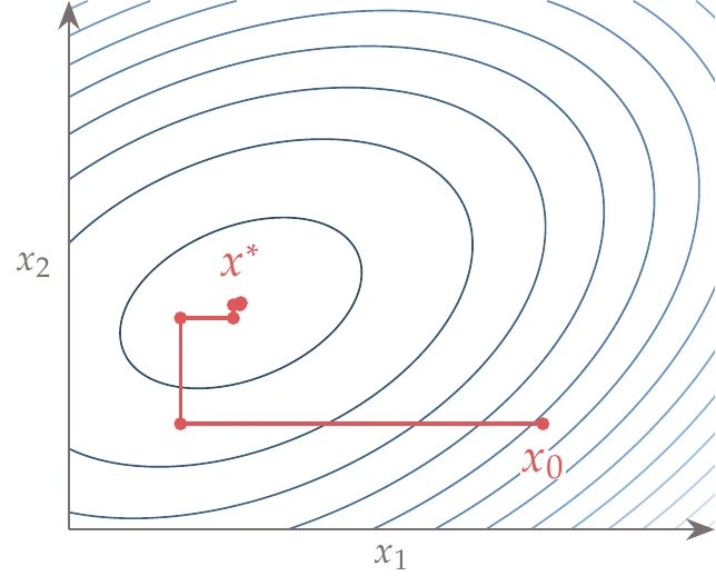
Figure 13.1:Sequential optimization is analogous to coordinate descent.
Sequential optimization is analogous to coordinate descent, which consists of optimizing each variable sequentially, as shown in Figure 13.1. Instead of optimizing one variable at a time, sequential optimization optimizes distinct sets of variables at a time, but the principle remains the same. This approach tends to work for unconstrained problems, although the convergence rate is limited to being linear.
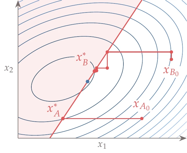
Figure 13.2:Sequential optimization can fail to find the constrained optimum because the optimization with respect to a set of variables might not see a feasible descent direction that otherwise exists when considering all variables simultaneously.
One issue with sequential optimization is that it might converge to a suboptimal point for a constrained problem. An example of such a case is shown in Figure 13.2, where sequential optimization gets stuck at the constraint because it cannot decrease the objective while remaining feasible by only moving in one of the directions. In this case, the optimization must consider both variables simultaneously to find a feasible descent direction.
Another issue is that when there are variables that affect multiple disciplines (called shared design variables), we must make a choice about which discipline handles those variables.
If we let each discipline optimize the same shared variable, the optimizations likely yield different values for those variables each time, in which case they will not converge. On the other hand, if we let one discipline handle a shared variable, it will likely converge to a value that violates one or more constraints from the other disciplines.
By considering the various components and optimizing a multidisciplinary performance metric with respect to as many design variables as possible simultaneously, MDO automatically finds the best trade-off between the components—this is the key principle of MDO. Suboptimal designs also result from decisions at the system level that involve power struggles between designers. In contrast, MDO provides the right trade-offs because mathematics does not care about politics.
In the absence of a coupled model, aerodynamicists may have to assume a fixed wing shape at the flight conditions of interest. Similarly, structural designers may assume fixed loads in their structural analysis. However, solving the coupled model is necessary to get the actual flying shape of the wing and the corresponding performance metrics.
One possible design optimization problem based on these models would be to minimize the drag by changing the wing shape and the structural sizing while satisfying a lift constraint and structural stress constraints.
Optimizing the wing shape and structural sizing simultaneously yields the best possible result because it finds feasible descent directions that would not be available with sequential optimization.
Wing shape variables, such as wingspan, are shared design variables because they affect both the aerodynamics and the structure. They cannot be optimized by considering aerodynamics or structures separately.
13.2 Coupled Models
As mentioned in Chapter 3, a model is a set of equations that we solve to predict the state of the engineering system and compute the objective and constraint function values. More generally, we can have a coupled model, which consists of multiple models (or components) that depend on each other’s state variables.
The same steps for formulating a design optimization problem (Section 1.2) apply in the formulation of MDO problems. The main difference in MDO problems is that the objective and constraints are computed by the coupled model. Once such a model is in place, the design optimization problem statement (Equation 1.4) applies, with no changes needed.
A generic example of a coupled model with three components is illustrated in Figure 13.4. Here, the states of each component affect all other components. However, it is common for a component to depend only on a subset of the other system components. Furthermore, we might distinguish variables between internal state variables and coupling variables (more in this in Section 13.2.2).
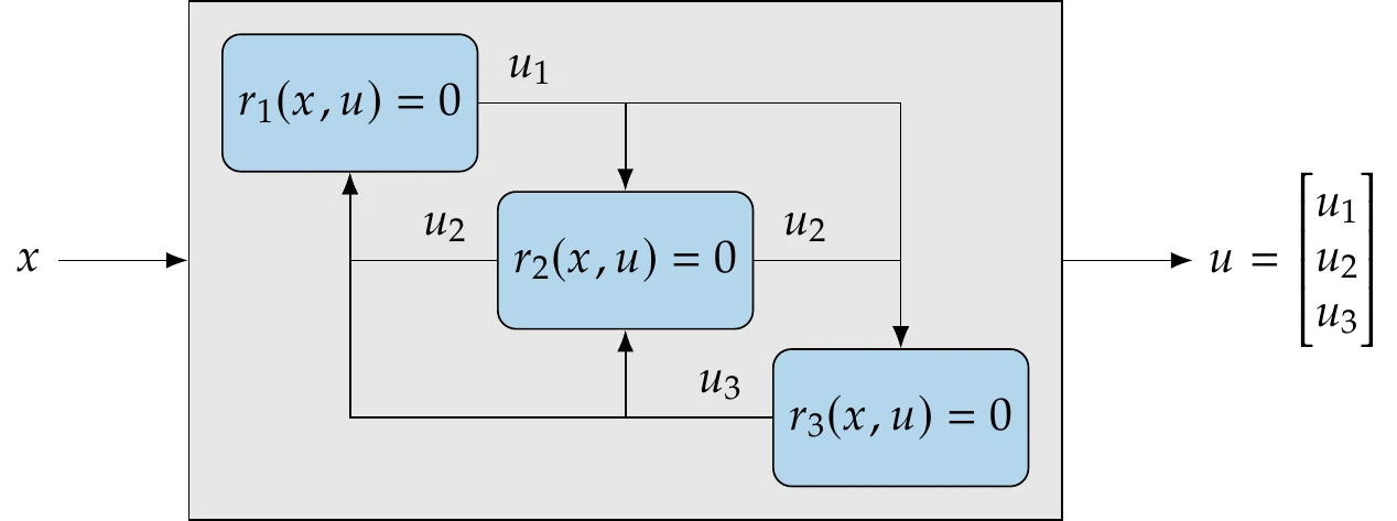
Figure 13.4:Coupled model composed of three numerical models. This coupled model would replace the single model in Figure 3.21.
Mathematically, a coupled model is no more than a larger set of equations to be solved, where all the governing equation residuals (), the corresponding state variables (), and all the design variables () are concatenated into single vectors. Then, we can still just write the whole multidisciplinary model as .
However, it is often necessary or advantageous to partition the system into smaller components for three main reasons. First, specialized solvers are often already in place for a given set of governing equations, which may be more efficient at solving their set of equations than a general-purpose solver. In addition, some of these solvers might be black boxes that do not provide an interface for using alternative solvers. Second, there is an incentive for building the multidisciplinary system in a modular way. For example, a component might be useful on its own and should therefore be usable outside the multidisciplinary system.
A modular approach also facilitates the extension of the multidisciplinary system and makes it easy to replace the model of a given discipline with an alternative one. Finally, the overall system of equations may be more efficiently solved if it is partitioned in a way that exploits the system structure. These reasons motivate an implementation of coupled models that is flexible enough to handle a mixture of different types of models and solvers for each component.
We start the remainder of this section by defining components in more detail (Section 13.2.1). We explain how the coupling variables relate to the state variables (Section 13.2.2) and coupled system formulation (Section 13.2.3). Then, we discuss the coupled system structure (Section 13.2.4). Finally, we explain methods for solving coupled systems (Section 13.2.5), including a hierarchical approach that can handle a mixture of models and solvers (Section 13.2.6).
13.2.1 Components
In Section 3.3, we explained how all models can ultimately be written as a system of residuals, . When the system is large or includes submodels, it might be natural to partition the system into components. We prefer to use the more general term components instead of disciplines to refer to the submodels resulting from the partitioning because the partitioning of the overall model is not necessarily by discipline (e.g., aerodynamics, structures). A system model might also be partitioned by physical system components (e.g., wing, fuselage, or an aircraft in a fleet) or by different conditions applied to the same model (e.g., aerodynamic simulations at different flight conditions).
The partitioning can also be performed within a given discipline for the same reasons cited previously. In theory, the system model equations in can be partitioned in any way, but only some partitions are advantageous or make sense.
We denote a partitioning into components as
Each and are vectors corresponding to the residuals and states of component . The semicolon denotes that we solve each component by driving its residuals () to zero by varying only its states () while keeping the states from all other components constant. We assume this is possible, but this is not guaranteed in general. We have omitted the dependency on in Equation 13.1 because, for now, we just want to find the state variables that solve the governing equations for a fixed design.
Components can be either implicit or explicit, a concept we introduced in Section 3.3. To solve an implicit component , we need an algorithm for driving the equation residuals, , to zero by varying the states while the other states ( for all ) remain fixed. This algorithm could involve a matrix factorization for a linear system or a Newton solver for a nonlinear system.
An explicit component is much easier to solve because that components’ states are explicit functions of other components’ states. The states of an explicit component can be computed without factorization or iteration. Suppose that the states of a component are given by the explicit function for all . As previously explained in Section 3.3, we can convert an explicit equation to the residual form by moving the function on the right-hand side to the left-hand side. Then, we obtain set of residuals,
Therefore, there is no loss of generality when using the residual notation in Equation 13.1.
Most disciplines involve a mix of implicit and explicit components because, as mentioned in Section 3.3 and shown in Figure 3.21, the state variables are implicitly defined, whereas the objective function and constraints are usually explicit functions of the state variables. In addition, a discipline usually includes functions that convert inputs and outputs, as discussed in Section 13.2.3.
As we will see in Section 13.2.6, the partitioning of a model can be hierarchical, where components are gathered in multiple groups. These groups can be nested to form a hierarchy with multiple levels. Again, this might be motivated by efficiency, modularity, or both.
13.2.2 Models and Coupling Variables
In MDO, the coupling variables are variables that need to be passed from the model of one discipline to the others because of interdependencies in the system. Thus, the coupling variables are the inputs and outputs of each model. Sometimes, the coupling variables are just the state variables of one model (or a subset of these) that get passed to another model, but often we need to convert between the coupling variables and other variables within the model.
We represent the coupling variables by a vector , where the subscript denotes the model that computes these variables. In other words, contains the outputs of model . A model can take any coupling variable vector as one of its inputs, where the subscript indicates that can be the output from any model except its own. Figure 13.7 shows the inputs and outputs for a model. The model solves for the set of its state variables, . The residuals in the solver depend on the input variables coming from other models. In general, this is not a direct dependency, so the model may require an explicit function () that converts the inputs () to the required parameters . These parameters remain fixed when the model solves its implicit equations for .
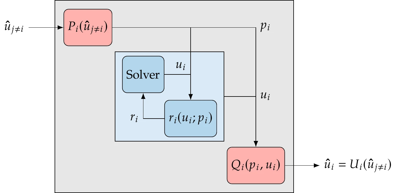
Figure 13.7:In the general case, a model may require conversions of inputs and outputs distinct from the states that the solver computes.
After the model solves for its state variables (), there may be another explicit function () that converts these states to output variables () for the other models. The function () typically reduces the number of output variables relative to the number of internal states, sometimes by orders of magnitude.
The model shown in Figure 13.7 can be viewed as an implicit function that computes its outputs as a function of all the inputs, so we can write . The model contains three components: two explicit and one implicit. We can convert the explicit components to residual equations using Equation 13.2 and express the model as three sets of residuals as shown in Figure 13.8. The result is a group of three components that we can represent as . This conversion and grouping hint at a powerful concept that we will use later, which is hierarchy, where components can be grouped using multiple levels.
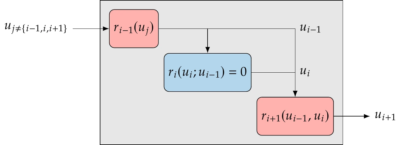
Figure 13.8:The conversion of inputs and outputs can be represented as explicit components with corresponding state variables. Using this form, any model can be entirely expressed as . The inputs could be any subset of except for those handled in the component (, , and ).
13.2.3 Residual and Functional Forms
The system-level representation of a coupled system is determined by the variables that are “seen” and controlled at this level.
Representing all models and variable conversions as leads to the residual form of the coupled system, already written in Equation 13.1, where is the number of components. In this case, the system level has direct access and control over all the variables. This residual form is desirable because, as we will see later in this chapter, it enables us to formulate efficient ways to solve coupled systems and compute their derivatives.
The functional form is an alternate system-level representation of the coupled system that considers only the coupling variables and expresses them as implicit functions of the others. We can write this form as
where is the number of models and . If a model is a black box and we have no access to the residuals and the conversion functions, this is the only form we can use. In this case, the system-level solver only iterates the coupling variables and relies on each model to solve or compute its outputs .
These two forms are shown in Figure 13.9 for a generic example with three models (or disciplines). The left of this figure shows the residual form, where each model is represented as residuals and states, as in Figure 13.8. This leads to a system with nine sets of residuals and corresponding state variables. The number of state variables in each of these sets is not specified but could be any number.
The functional form of these three models is shown on the right of Figure 13.9. In the case where the model is a black box, the residuals and conversion functions shown in Figure 13.7 are hidden, and the system level can only access the coupling variables. In this case, each black-box is considered to be a component, as shown in the right of Figure 13.9.
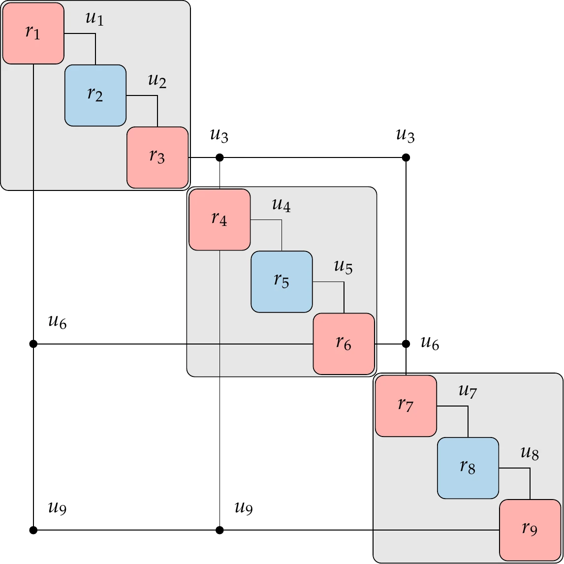
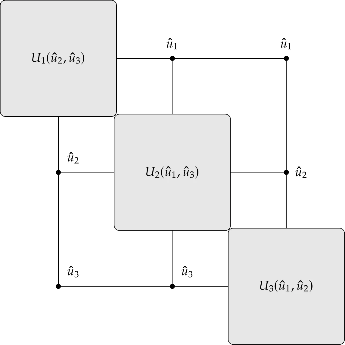
Figure 13.9:Two system-level views of coupled system with three solvers. In the residual form, all components and their states are exposed (a); in the functional (black-box) form, only inputs and outputs for each solver are visible (b), where , , and . (a) Residual form. (b) Functional form.
In an even more general case, these two views can be mixed in a coupled system. The models in residual form expose residuals and states, in which case, the model potentially has multiple components at the system level. The models in functional form only expose inputs and outputs; in that case, the model is just a single component.
13.2.4 Coupled System Structure
To show how multidisciplinary systems are coupled, we use a design structure matrix (DSM), which is sometimes referred to as a dependency structure matrix or an matrix. An example of the DSM for a hypothetical system is shown on the left in Figure 13.10. In this matrix, the diagonal elements represent the components, and the off-diagonal entries denote coupling variables. A given coupling variable is computed by the component in its row and is passed to the component in its column.[2]As shown in the DSM on the left side of Figure 13.10, there are generally off-diagonal entries both above and below the diagonal, where the entries above feed forward, whereas entries below feed backward.
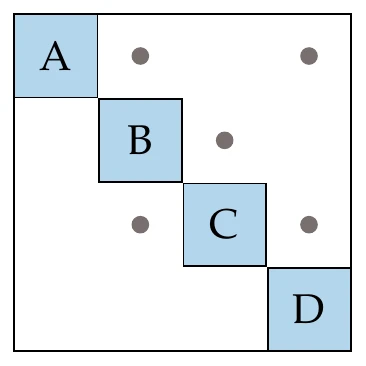
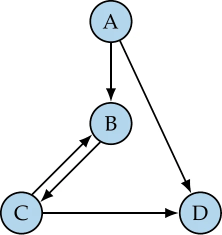
Figure 13.10:Different ways to represent the dependencies of a hypothetical coupled system.
The mathematical representation of these dependencies is given by a graph (Figure 13.10, right), where the graph nodes are the components, and the edges represent the information dependency. This graph is a directed graph because, in general, there are three possibilities for coupling two components: single coupling one way, single coupling the other way, and two-way coupling. A directed graph is cyclic when there are edges that form a closed loop (i.e., a cycle). The graph on the right of Figure 13.10 has a single cycle between components B and C. When there are no closed loops, the graph is acyclic. In this case, the whole system can be solved by solving each component in turn without iterating.
The DSM can be viewed as a matrix where the blank entries are zeros. For real-world systems, this is often a sparse matrix. This means that in the corresponding DSM, each component depends only on a subset of all the other components. We can take advantage of the structure of this sparsity in the solution of coupled systems.
The components in the DSM can be reordered without changing the solution of the system. This is analogous to reordering sparse matrices to make linear systems easier to solve. In one extreme case, reordering could achieve a DSM with no entries below the diagonal. In that case, we would have only feedforward connections, which means all dependencies could be resolved in one forward pass (as we will see in Example 13.4). This is analogous to having a linear system where the matrix is lower triangular, in which case the linear solution can be obtained with forward substitution.
The sparsity of the DSM can be exploited using ideas from sparse linear algebra. For example, reducing the bandwidth of the matrix (i.e., moving nonzero elements closer to the diagonal) can also be helpful. This can be achieved using algorithms such as Cuthill–McKee,2 reverse Cuthill–McKee (RCM), and approximate minimum degree (AMD) ordering.3[3]We now introduce an extended version of the DSM, called XDSM,4 which we use later in this chapter to show the process in addition to the data dependencies. Figure 13.11 shows the XDSM for the same four-component system. When showing only the data dependencies, the only difference relative to DSM is that the coupling variables are labeled explicitly, and the data paths are drawn. In the next section, we add the process to the XDSM.
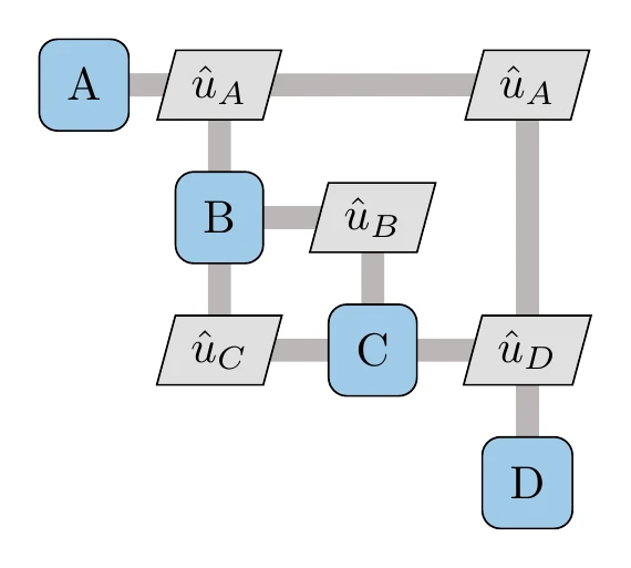
Figure 13.11:XDSM showing data dependencies for the four-component coupled system of Figure 13.10.
13.2.5 Solving Coupled Numerical Models
The solution of coupled systems, also known as multidisciplinary analysis (MDA), requires concepts beyond the solvers reviewed in Section 3.6 because it usually involves multiple levels of solvers.
When using the residual form described in Section 13.2.3, any solver (such as a Newton solver) can be used to solve for the state of all components (the entire vector ) simultaneously to satisfy for the coupled system (Equation 13.1). This is a monolithic solution approach.
When using the functional form, we do not have access to the internal states of each model and must rely on the model’s solvers to compute the coupling variables. The model solver is responsible for computing its output variables for a given set of coupling variables from other models, that is,
In some cases, we have access to the model’s internal states, but we may want to use a dedicated solver for that model anyway.
Because each model, in general, depends on the outputs of all other models, we have a coupled dependency that requires a solver to resolve. This means that the functional form requires two levels: one for the model solvers and another for the system-level solver. At the system level, we only deal with the coupling variables (), and the internal states () are hidden.
The rest of this section presents several system-level solvers. We will refer to each model as a component even though it is a group of components in general.
Nonlinear Block Jacobi
The most straightforward way to solve coupled numerical models (systems of components) is through a fixed-point iteration, which is analogous to the fixed-point iteration methods mentioned in Section 3.6 and detailed in Section B.4.1. The difference here is that instead of updating one state at a time, we update a vector of coupling variables at each iteration corresponding to a subset of the coupling variables in the overall coupled system. Obtaining this vector of coupling variables generally involves the solution of a nonlinear system. Therefore, these are called nonlinear block variants of the linear fixed-point iteration methods.
The nonlinear block Jacobi method requires an initial guess for all coupling variables to start with and calls for the solution of all components given those guesses. Once all components have been solved, the coupling variables are updated based on the new values computed by the components, and all components are solved again. This iterative process continues until the coupling variables do not change in subsequent iterations. Because each component takes the coupling variable values from the previous iteration, which have already been computed, all components can be solved in parallel without communication.
This algorithm is formalized in Algorithm 13.1. When applied to a system of components, we call it the block Jacobi method, where block refers to each component.
The nonlinear block Jacobi method is also illustrated using an XDSM in Figure 13.12 for three components. The only input is the initial guess for the coupling variables, .[4]The MDA block (step 0) is responsible for iterating the system-level analysis loop and for checking if the system has converged. The process line is shown as a thin black line to distinguish it from the data dependency connections (thick gray lines) and follows the sequence of numbered steps. The analyses for each component are all numbered the same (step 1) because they can be done in parallel. Each component returns the coupling variables it computes to the MDA iterator, closing the loop between step 2 and step 1 (denoted as “”).
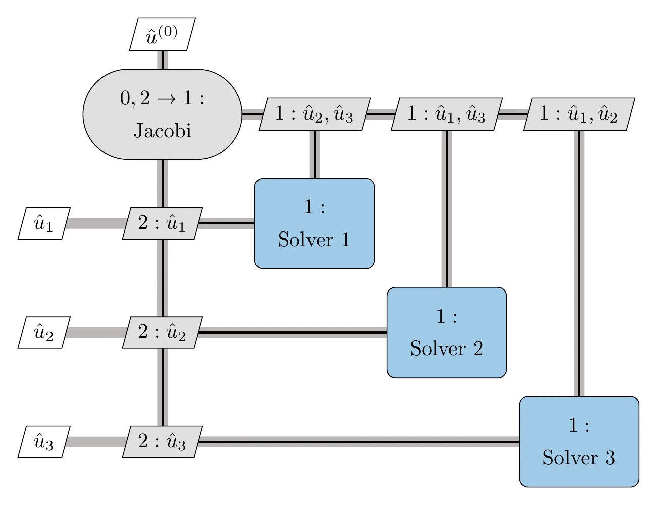
Figure 13.12:Nonlinear block Jacobi solver for a three-component coupled system.
The block Jacobi solver (Algorithm 13.1) can also be used when one or more components are linear solvers. This is useful for computing the derivatives of the coupled system using implicit analytics methods because that involves solving a coupled linear system with the same structure as the coupled model (see Section 13.3.3).
Nonlinear Block Gauss–Seidel
The nonlinear block Gauss–Seidel algorithm is similar to its Jacobi counterpart. The only difference is that when solving each component, we use the latest coupling variables available instead of just using the coupling variables from the previous iteration.
We cycle through each component in order. When computing by solving component , we use the latest available states from the other components.
Figure 13.13 illustrates this process.
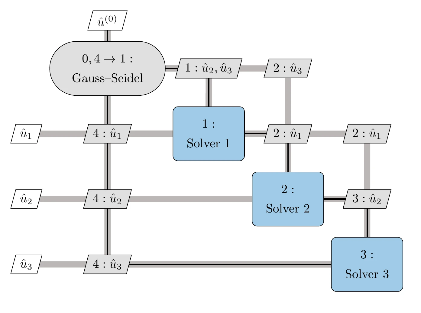
Figure 13.13:Nonlinear block Gauss–Seidel solver for the three-discipline coupled system of Figure 13.9.
Both Gauss–Seidel and Jacobi converge linearly, but Gauss–Seidel tends to converge more quickly because each equation uses the latest information available. However, unlike Jacobi, the components can no longer be solved in parallel.
The convergence of nonlinear block Gauss–Seidel can be improved by using a relaxation. Suppose that is the state of component resulting from the solving of that component given the states of all other components, as we would normally do for each block in the Gauss–Seidel or Jacobi method.
If we used this, the step would be
Instead of using that step, relaxation updates the variables as
where is the relaxation factor, and is the previous update for component . The relaxation factor, , could be a fixed value, which would normally be less than 1 to dampen oscillations and avoid divergence.
Aitken’s method5 improves on the fixed relaxation approach by adapting the . The relaxation factor at each iteration changes based on the last two updates according to
Aitken’s method usually accelerates convergence and has been shown to work well for nonlinear block Gauss–Seidel with multidisciplinary systems.6 It is advisable to override the value of the relaxation factor given by Equation 13.8 to keep it between 0.25 and 2.7
The steps for the full Gauss–Seidel algorithm with Aitken acceleration are listed in Algorithm 13.2. Similar to the block Jacobi solver, the block Gauss–Seidel solver can also be used when one or more components are linear solvers. Aitken acceleration can be used in the linear case without modification and it is still useful.
The order in which the components are solved makes a significant difference in the efficiency of the Gauss–Seidel method. In the best possible scenario, the components can be reordered such that there are no entries in the lower diagonal of the DSM, which means that each component depends only on previously solved components, and there are therefore no feedback dependencies (see Example 13.4).
In this case, the block Gauss–Seidel method would converge to the solution in one forward sweep.
In the more general case, even though we might not eliminate the lower diagonal entries completely, minimizing these entries by reordering results in better convergence. This reordering can also mean the difference between convergence and nonconvergence.
Newton’s Method
As mentioned previously, Newton’s method can be applied to the residual form illustrated in Figure 13.9 and expressed in Equation 13.1. Recall that in this form, we have components and the coupling variables are part of the state variables. In this case, Newton’s method is as described in Section 3.8.
Concatenating the residuals and state variables for all components and applying Newton’s method yields the coupled block Newton system,
We can solve this linear system to compute the Newton step for all components’ state variables simultaneously, and then iterate to satisfy for the complete system.
This is the monolithic Newton approach illustrated on the left panel of Figure 13.15. As with any Newton method, a globalization strategy (such as a line search) is required to increase the likelihood of successful convergence when starting far from the solution (see Section 4.2). Even with such a strategy, Newton’s method does not necessarily converge robustly.
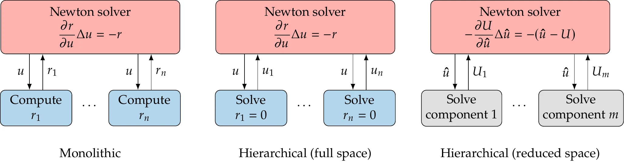
Figure 13.15:There are three options for solving a coupled system with Newton’s method. The monolithic approach (left) solves for all state variables simultaneously. The block approach (middle) solves the same system as the monolithic approach, but solves each component for its states at each iteration. The black box approach (right) applies Newton’s method to the coupling variables.
A variation on this monolithic Newton approach uses two-level solver hierarchy, as illustrated on the middle panel of Figure 13.15. The system-level solver is the same as in the monolithic approach, but each component is solved first using the latest states. The Newton step for each component is given by
where represents the states from other components (i.e., ), which are fixed at this level. Each component is solved before taking a step in the entire state vector (Equation 13.9). The procedure is given in Algorithm 13.3 and illustrated in Figure 13.16. We call this the full-space hierarchical Newton approach because the system-level solver iterates the entire state vector. Solving each component before taking each step in the full space Newton iteration acts as a preconditioner. In general, the monolithic approach is more efficient, and the hierarchical approach is more robust, but these characteristics are case-dependent.

Figure 13.16:Full-space hierarchical Newton solver for a three-component coupled system.
Newton’s method can also be applied to the functional form illustrated in Figure 13.9 to solve only for the coupling variables. We call this the reduced-space hierarchical Newton approach because the system-level solver iterates only in the space of the coupling variables, which is smaller than the full space of the state variables. Using this approach, each component’s solver can be a black box, as in the nonlinear block Jacobi and Gauss–Seidel solvers. This approach is illustrated on the right panel of Figure 13.15. The reduced-space approach is mathematically equivalent and follows the same iteration path as the full-space approach if each component solver in the reduced-space approach is converged well enough.8
To apply the reduced-space Newton’s method, we express the functional form (Equation 13.4) as residuals by using the same technique we used to convert an explicit function to the residual form (Equation 13.2). This yields
where represents the guesses for the coupling variables, and represents the actual computed values. For a system of nonlinear residual equations, the Newton step in the coupling variables, , can be found by solving the linear system
where we need the partial derivatives of all the residuals with respect to the coupling variables to form the Jacobian matrix . The Jacobian can be found by differentiating Equation 13.11 with respect to the coupling variables. Then, expanding the concatenated residuals and coupling variable vectors yields
The residuals in the right-hand side of this equation are evaluated at the current iteration.
The derivatives in the block Jacobian matrix are also computed at the current iteration. Each row represents the derivatives of the (potentially implicit) function that computes the outputs of component with respect to all the inputs of that component. The Jacobian matrix in Equation 13.13 has the same structure as the DSM (but transposed) and is often sparse. These derivatives can be computed using the methods from Chapter 6. These are partial derivatives in the sense that they do not take into account the coupled system. However, they must take into account the respective model and can be computed using implicit analytic methods when the model is implicit.
This Newton solver is shown in Figure 13.17 and detailed in Algorithm 13.4. Each component corresponds to a set of rows in the block Newton system (Equation 13.13). To compute each set of rows, the corresponding component must be solved, and the derivatives of its outputs with respect to its inputs must be computed as well. Each set can be computed in parallel, but once the system is assembled, a step in the coupling variables is computed by solving the full system (Equation 13.13).
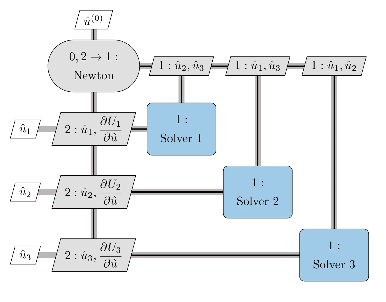
Figure 13.17:Reduced-space hierarchical Newton solver for a three-component coupled system.
These coupled Newton methods have similar advantages and disadvantages to the plain Newton method. The main advantage is that it converges quadratically once it is close enough to the solution (if the problem is well-conditioned). The main disadvantage is that it might not converge at all, depending on the initial guess. One disadvantage specific to the coupled Newton methods is that it requires formulating and solving the coupled linear system (Equation 13.13) at each iteration.
If the Jacobian is not readily available, Broyden’s method can approximate the Jacobian inverse () by starting with a guess (say, ) and then using the update
where is the last step in the states and is the difference between the two latest residual vectors. Because the inverse is provided explicitly, we can find the update by performing the multiplication,
Broyden’s method is analogous to the quasi-Newton methods of Section 4.4.4 and is derived in Section C.1.
13.2.6 Hierarchical Solvers for Coupled Systems
The coupled solvers we discussed so far already use a two-level hierarchy because they require a solver for each component and a second level that solves the group of components. This hierarchy can be extended to three and more levels by making groups of groups.
Modular analysis and unified derivatives (MAUD) is a mathematical framework developed for this purpose. Using MAUD, we can mix residual and functional forms and seamlessly handle implicit and explicit components.[6]
The hierarchy of solvers can be represented as a tree data structure, where the nodes are the solvers and the leaves are the components, as shown in Figure 13.20 for a system of six components and five solvers. The root node ultimately solves the complete system, and each solver is responsible for a subsystem and thus handles a subset of the variables.
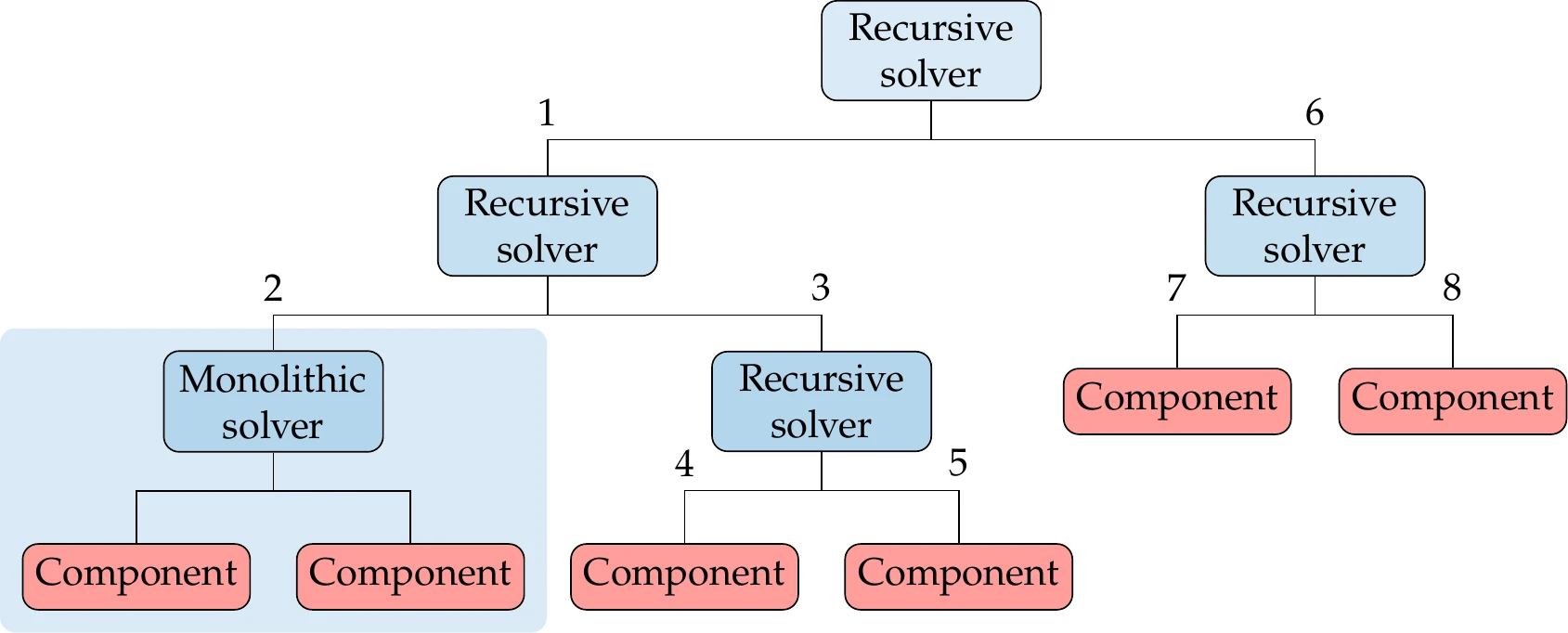
Figure 13.20:A system of components can be organized in a solver hierarchy.
There are two possible types of solvers: monolithic and recursive. Monolithic solvers can only have components as children and handle all their variables simultaneously using the residual form. Of the methods we introduced in the previous section, only monolithic and full-space Newton (and Broyden) can do this for nonlinear systems. Linear systems can be solved in a monolithic fashion using a direct solver or an iterative linear solver, such as a Krylov subspace method. Recursive solvers, as the name implies, visit all the child nodes in turn. If a child node turns out to be another recursive solver, it does the same until a component is reached. The block Jacobi and Gauss–Seidel methods can be used as recursive solvers for nonlinear and linear systems. The reduced-space Newton and Broyden methods can also be recursive solvers.
For the hypothetical system shown in Figure 13.20, the numbers show the order in which each solver and component would be called.
The hierarchy of solvers should be chosen to exploit the system structure. MAUD also facilitates parallel computation when subsystems are uncoupled, which provides further opportunities to exploit the structure of the problem. Figure 13.21 and Figure 13.22 show several possibilities.
The three systems in Figure 13.21 show three different coupling modes. In the first mode, the two components are independent of each other and can be solved in parallel using any solvers appropriate for each of the components. In the serial case, component 2 depends on 1, but not the other way around. Therefore, we can converge to the coupled solution using one block Gauss–Seidel iteration. If the dependency were reversed (feedback but no feedforward), the order of the two components would be switched. Finally, the fully coupled case requires an iterative solution using any of the methods from Section 13.2.5. MAUD is designed to handle these three coupling modes.
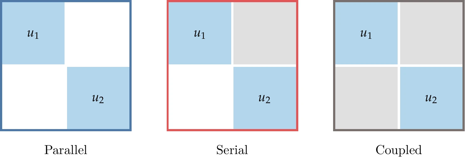
Figure 13.21:There are three main possibilities involving two components.
Figure 13.22 shows three possibilities for a four-component system where two levels of solvers can be used. In the first one (on the left), we require a coupled solver for components 1 and 2 and another for components 3 and 4, but no further solving is needed. In the second (Figure 13.22, middle), components 1 and 2 as well as components 3 and 4 can be solved serially, but these two groups require a coupled solution. For the two levels to converge, the serial and coupled solutions are called repeatedly until the two solvers agree with each other.
The third possibility (Figure 13.22, right) has two systems that have two independent components, which can each be solved in parallel, but the overall system is coupled. With MAUD, we can set up any of these sequences of solvers through the solver hierarchy tree, as illustrated in Figure 13.20.
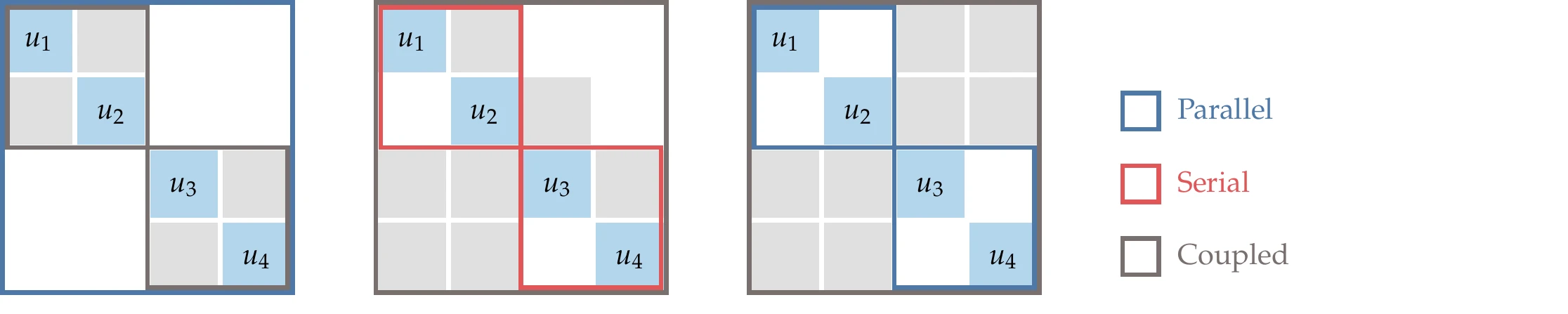
Figure 13.22:Three examples of a system of four components with a two-level solver hierarchy.
To solve the system from Example 13.3 using hierarchical solvers, we can use the hierarchy shown in Figure 13.23. We form three groups with three components each. Each group includes the input and output conversion components (which are explicit) and one implicit component (which requires its own solver). Serial solvers can be used to handle the input and output conversion components. A coupled solver is required to solve the entire coupled system, but the coupling between the groups is restricted to the corresponding outputs (components 3, 6, and 9).
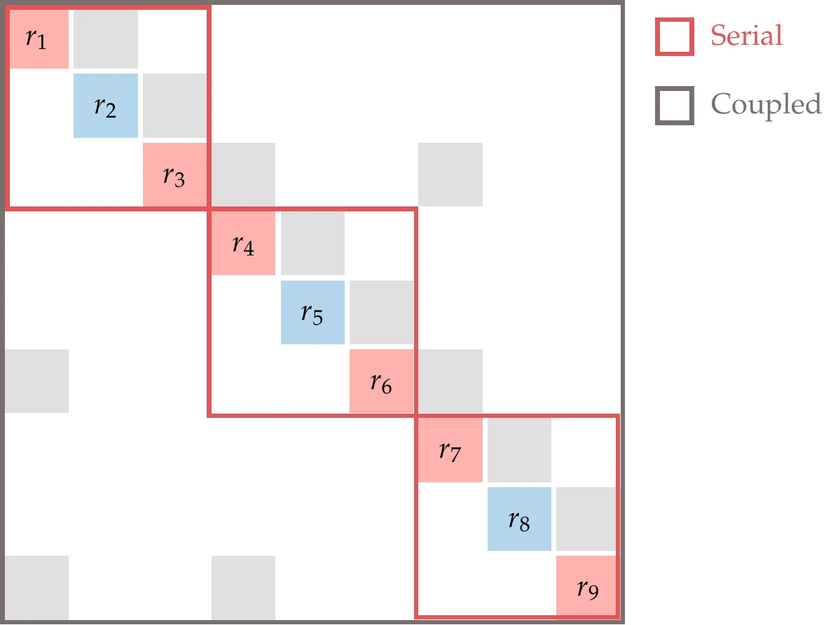
Figure 13.23:For the case of Figure 13.9, we can use a serial evaluation within each of the three groups and require a coupled solver to handle the coupling between the three groups.
Alternatively, we could apply a coupled solver to the functional representation (Figure 13.9, right). This would also use two levels of solvers: a solver within each group and a system-level solver for the coupling of the three groups. However, the system-level solver would handle coupling variables rather than the residuals of each component.
13.3 Coupled Derivatives Computation
The gradient-based optimization algorithms from Chapter 4 and Chapter 5 require the derivatives of the objective and constraints with respect to the design variables. Any of the methods for computing derivatives from Chapter 6 can be used to compute the derivatives of coupled models, but some modifications are required. The main difference is that in MDO, the computation of the functions of interest (objective and constraints) requires the solution of the multidisciplinary model.
13.3.1 Finite Differences
The finite-difference method can be used with no modification, as long as an MDA is converged well enough for each perturbation in the design variables. As explained in Section 6.4, the cost of computing derivatives with the finite-difference method is proportional to the number of variables. The constant of proportionality can increase significantly compared with that of a single discipline because the MDA convergence might be slow (especially if using a block Jacobi or Gauss–Seidel iteration).
The accuracy of finite-difference derivatives depends directly on the accuracy of the functions of interest. When the functions are computed from the solution of a coupled system, their accuracy depends both on the accuracy of each component and the accuracy of the MDA. To address the latter, the MDA should be converged well enough.
13.3.2 Complex Step and AD
The complex-step method and forward-mode AD can also be used for a coupled system, but some modifications are required. The complex-step method requires all components to be able to take complex inputs and compute the corresponding complex outputs. Similarly, AD requires inputs and outputs that include derivative information. For a given MDA, if one of these methods is applied to each component and the coupling includes the derivative information, we can compute the derivatives of the coupled system.
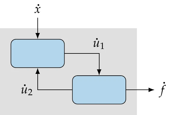
Figure 13.24:Forward mode of AD for a system of two components.
The propagation of the forward-mode seed (or the complex step) is illustrated in Figure 13.24 for a system of two components.
When using AD, manual coupling is required if the components and the coupling are programmed in different languages. The complex-step method can be more straightforward to implement than AD for cases where the models are implemented in different languages, and all the languages support complex arithmetic. Although both of these methods produce accurate derivatives for each component, the accuracy of the derivatives for the coupled system could be compromised by a low level of convergence of the MDA.
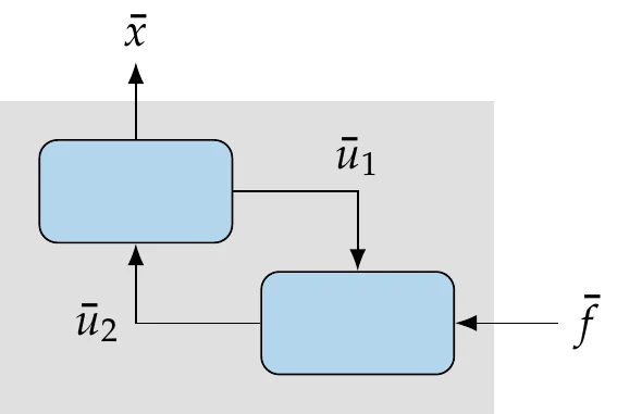
Figure 13.25:Reverse mode of AD for a system of two components.
The reverse mode of AD for coupled systems would be more involved: after an initial MDA, we would run a reverse MDA to compute the derivatives, as illustrated in Figure 13.25.
13.3.3 Implicit Analytic Methods
The implicit analytic methods from Section 6.7 (both direct and adjoint) can also be extended to compute the derivatives of coupled systems. All the equations derived for a single component in Section 6.7 are valid for coupled systems if we concatenate the residuals and the state variables. Furthermore, we can mix explicit and implicit components using concepts introduced in the UDE. Finally, when using the MAUD approach, the coupled derivative computation can be done using the same hierarchy of solvers.
Coupled Derivatives of Residual Representation
In Equation 13.1, we denoted the coupled system as a series of concatenated residuals, , and variables corresponding to each component as
where the residual for each component, , could depend on all states . To derive the coupled version of the direct and adjoint methods, we apply them to the concatenated vectors. Thus, the coupled version of the linear system for the direct method (Equation 6.43) is
where represents the derivatives of the states from component with respect to the design variables. Once we have solved for , we can use the coupled equivalent of the total derivative equation (Equation 6.44) to compute the derivatives:
Similarly, the adjoint equations (Equation 6.46) can be written for a coupled system using the same concatenated state and residual vectors. The coupled adjoint equations involve a corresponding concatenated adjoint vector and can be written as
After solving this equations for the coupled-adjoint vector, we can use the coupled version of the total derivative equation (Equation 6.47) to compute the desired derivatives as
Like the adjoint method from Section 6.7, the coupled adjoint is a powerful approach for computing gradients with respect to many design variables.[7]
The required partial derivatives are the derivatives of the residuals or outputs of each component with respect to the state variables or inputs of all other components. In practice, the block structure of these partial derivative matrices is sparse, and the matrices themselves are sparse. This sparsity can be exploited using graph coloring to drastically reduce the computation effort of computing Jacobians at the system or component level, as explained in Section 6.8.
Figure 13.26 shows the structure of the Jacobians in Equation 13.17 and Equation 13.19 for the three-group case from Figure 13.23. The sparsity structure of the Jacobian is the transpose of the DSM structure. Because the Jacobian in Equation 13.19 is transposed, the Jacobian in the adjoint equation has the same structure as the DSM.
The structure of the linear system can be exploited in the same way as for the nonlinear system solution using hierarchical solvers: serial solvers within each group and a coupled solver for the three groups. The block Jacobi and Gauss–Seidel methods from Section 13.2.5 are applicable to coupled linear components, so these methods can be re-used to solve this coupled linear system for the total coupled derivatives.
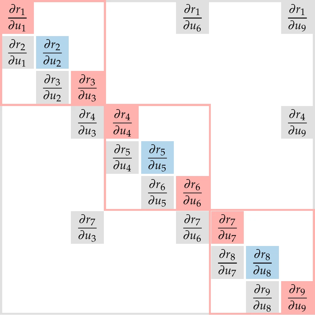
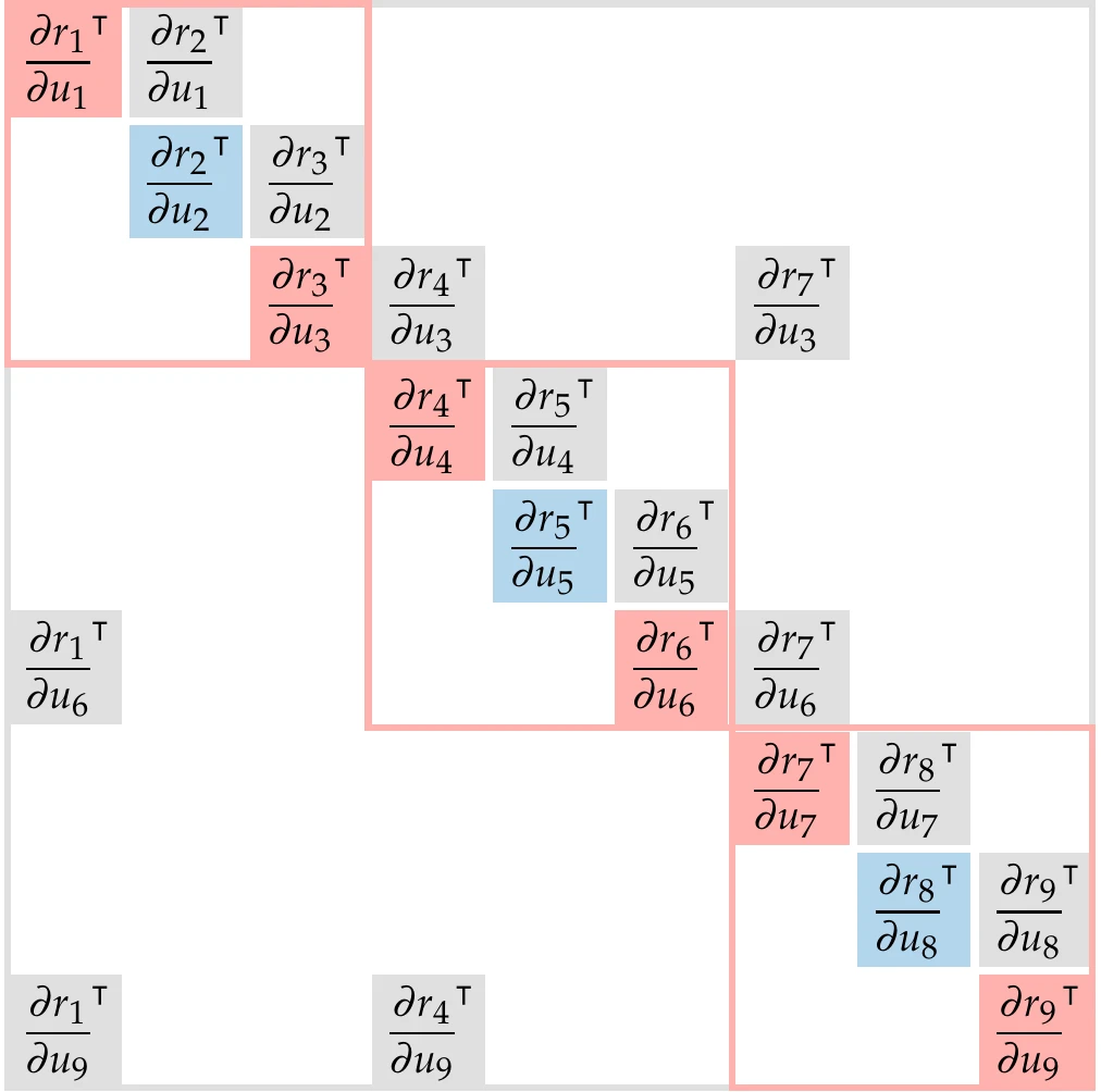
Figure 13.26:Jacobian structure for residual form of the coupled direct (a) and adjoint (b) equations for the three-group system of Figure 13.23. The structure of the transpose of the Jacobian is the same as that of the DSM. (a) Direct Jacobian. (b) Adjoint Jacobian.
The partial derivatives in the coupled Jacobian, the right-hand side of the linear systems (Equation 13.17 and Equation 13.19), and the total derivatives equations (Equation 13.18 and Equation 13.20) can be computed with any of the methods from Chapter 6. The nature of these derivatives is the same as we have seen previously for implicit analytic methods (Section 6.7). They do not require the solution of the equation and are typically cheap to compute. Ideally, the components would already have analytic derivatives of their outputs with respect to their inputs, which are all the derivatives needed at the system level.
The partial derivatives can also be computed using the finite-difference or complex-step methods. Even though these are not efficient for cases with many inputs, it might still be more efficient to compute the partial derivatives with these methods and then solve the coupled derivative equations instead of performing a finite difference of the coupled system, as described in Section 13.3.1. The reason is that computing the partial derivatives avoids having to reconverge the coupled system for every input perturbation. In addition, the coupled system derivatives should be more accurate when finite differences are used only to compute the partial derivatives.
Coupled Derivatives of Functional Representation
Variants of the coupled direct and adjoint methods can also be derived for the functional form of the system-level representation (Equation 13.4), by using the residuals defined for the system-level Newton solver (Equation 13.11),
Recall that driving these residuals to zero relies on a solver for each component to solve for each component’s states and another solver to solve for the coupling variables .
Using this new residual definition and the coupling variables, we can derive the functional form of the coupled direct method as
where the Jacobian is identical to the one we derived for the coupled Newton step (Equation 13.13). Here, represents the derivatives of the coupling variables from component with respect to the design variables. The solution can then be used in the following equation to compute the total derivatives:
Similarly, the functional version of the coupled adjoint equations can be derived as
After solving for the coupled-adjoint vector using the previous equation, we can use the total derivative equation to compute the desired derivatives:
Because the coupling variables () are usually a reduction of the internal state variables (), the linear systems in Equation 13.22 and Equation 13.24 are usually much smaller than that of the residual counterparts (Equation 13.17 and Equation 13.19). However, unlike the partial derivatives in the residual form, the partial derivatives in the functional form Jacobian need to account for the solution of the corresponding component. When viewed at the component level, these derivatives are actually total derivatives of the component. When the component is an implicit set of equations, computing these derivatives with finite-differencing would require solving the component’s equations for each variable perturbation. Alternatively, an implicit analytic method (from Section 6.7) could be applied to the component to compute these derivatives.
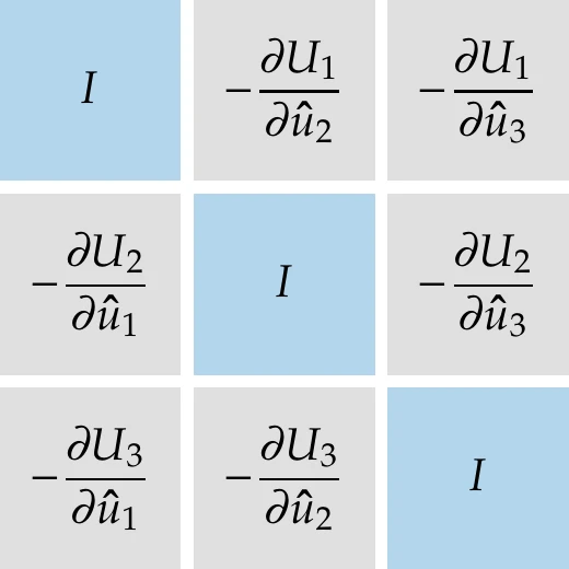
Figure 13.27:Jacobian of coupled derivatives for the functional form of Figure 13.23.
Figure 13.27 shows the Jacobian structure in the functional form of the coupled direct method (Equation 13.22) for the case of Figure 13.23. The dimension of this Jacobian is smaller than that of the residual form. Recall from Figure 13.9 that corresponds to , corresponds to , and corresponds to . Thus, the total size of this Jacobian corresponds to the sum of the sizes of components 3, 6, and 9, as opposed to the sum of the sizes of all nine components for the residual form. However, as mentioned previously, partial derivatives for the functional form are more expensive to compute because they need to account for an implicit solver in each of the three groups.
UDE for Coupled Systems
As in the single-component case in Section 6.9, the coupled direct and adjoint equations derived in this section can be obtained from the UDE with the appropriate definitions of residuals and variables. The components corresponding to each block in these equations can also be implicit or explicit, which provides the flexibility to represent systems of heterogeneous components.
MAUD implements the linear systems from these coupled direct and adjoint equations using the UDE. The overall linear system inherits the hierarchical structure defined for the nonlinear solvers. Instead of nonlinear solvers, we use linear solvers, such as a direct solver and Krylov (both monolithic). As mentioned in Section 13.2.5, the nonlinear block Jacobi and Gauss–Seidel (both recursive) can be reused to solve coupled linear systems. Components can be expressed using residual or functional forms, making it possible to include black-box components.
The example originally used in Chapter 6 to demonstrate how to compute derivatives with the UDE (Example 6.15) can be viewed as a coupled derivative computation where each equation is a component. Example 13.6 demonstrates the UDE approach to computing derivatives by building on the wing design problem presented in Example 13.2.
13.4 Monolithic MDO Architectures
So far in this chapter, we have extended the models and solvers from Chapter 3 and derivative computation methods from Chapter 6 to coupled systems. We now discuss the options to optimize coupled systems, which are given by various MDO architectures.
Monolithic MDO architectures cast the design problem as a single optimization. The only difference between the different monolithic architectures is the set of design variables that the optimizer is responsible for, which affects the constraint formulation and how the governing equations are solved.
13.4.1 Multidisciplinary Feasible
The multidisciplinary design feasible (MDF) architecture is the architecture that is most similar to a single-discipline problem and usually the most intuitive for engineers. The design variables, objective, and constraints are the same as we would expect for a single-discipline problem. The only difference is that the computation of the objective and constraints requires solving a coupled system instead of a single system of governing equations. Therefore, all the optimization algorithms covered in the previous chapters can be applied without modification when using the MDF architecture. This approach is also called a reduced-space approach because the optimizer does not handle the space of the state and coupling variables. Instead, it relies on a solver to find the state variables that satisfy the governing equations for the current design (see Equation 3.32).
The resulting optimization problem is as follows:[9]
At each optimization iteration, the optimizer has a multidisciplinary feasible point found through the MDA. For a design given by the optimizer (), the MDA finds the internal component states () and the coupling variables (). To denote the MDA solution, we use the residuals of the functional form, where the residuals for component are[10]
Each component is assumed to solve for its state variables internally. The MDA finds the coupling variables by solving the coupled system of components using one of the methods from Section 13.2.5.
Then, the objective and constraints can be computed based on the current design variables and coupling variables. Figure 13.30 shows an XDSM for MDF with three components. Here we use a nonlinear block Gauss–Seidel method (see Algorithm 13.2) to converge the MDA, but any other method from Section 13.2.5 could be used.
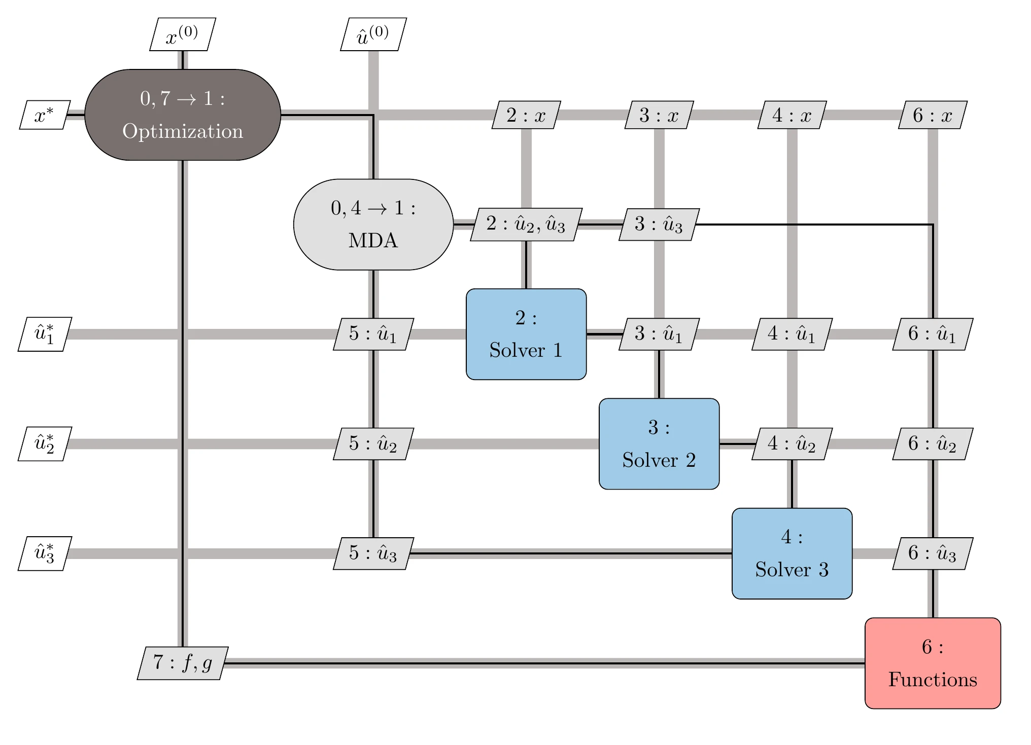
Figure 13.30:The MDF architecture relies on an MDA to solve for the coupling and state variables at each optimization iteration. In this case, the MDA uses the block Gauss–Seidel method.
One advantage of MDF is that the system-level states are physically compatible if an optimization stops prematurely. This is advantageous in an engineering design context when time is limited, and we are not as concerned with finding an optimal design in the strict mathematical sense as we are with finding an improved design. However, it is not guaranteed that the design constraints are satisfied if the optimization is terminated early; that depends on whether the optimization algorithm maintains a feasible design point or not.
The main disadvantage of MDF is that it solves an MDA for each optimization iteration, which requires its own algorithm outside of the optimization. Implementing an MDA algorithm can be time-consuming if one is not already in place.
As mentioned in Tip 13.3, a MAUD-based framework such as OpenMDAO can facilitate this. MAUD naturally implements the MDF architecture because it focuses on solving the MDA (Section 13.2.5) and on computing the derivatives corresponding to the MDA (Section 13.3.3).[11]
When using a gradient-based optimizer, gradient computations are also challenging for MDF because coupled derivatives are required. Finite-difference derivative approximations are easy to implement, but their poor scalability and accuracy are compounded by the MDA, as explained in Section 13.3. Ideally, we would use one of the analytic coupled derivative computation methods of Section 13.3, which require a substantial implementation effort. Again, OpenMDAO was developed to facilitate coupled derivative computation (see Tip 13.4).
13.4.2 Individual Discipline Feasible
The individual discipline feasible (IDF) architecture adds independent copies of the coupling variables to allow component solvers to run independently and possibly in parallel. These copies are known as target variables and are controlled by the optimizer, whereas the actual coupling variables are computed by the corresponding component. Target variables are denoted by a superscript , so the coupling variables produced by discipline are denoted as . These variables represent the current guesses for the coupling variables that are independent of the corresponding actual coupling variables computed by each component. To ensure the eventual consistency between the target coupling variables and the actual coupling variables at the optimum, we define a set of consistency constraints, , which we add to the optimization problem formulation.
The optimization problem for the IDF architecture is
Each component is solved independently to compute the corresponding output coupling variables , where the inputs are given by the optimizer. Thus, each component drives its residuals to zero to compute
The consistency constraint quantifies the difference between the target coupling variables guessed by the optimizer and the actual coupling variables computed by the components. The optimizer iterates the target coupling variables simultaneously with the design variables to find a multidisciplinary feasible point that is also an optimum. At each iteration, the objective and constraints are computed using the latest available coupling variables. Figure 13.35 shows the XDSM for IDF.
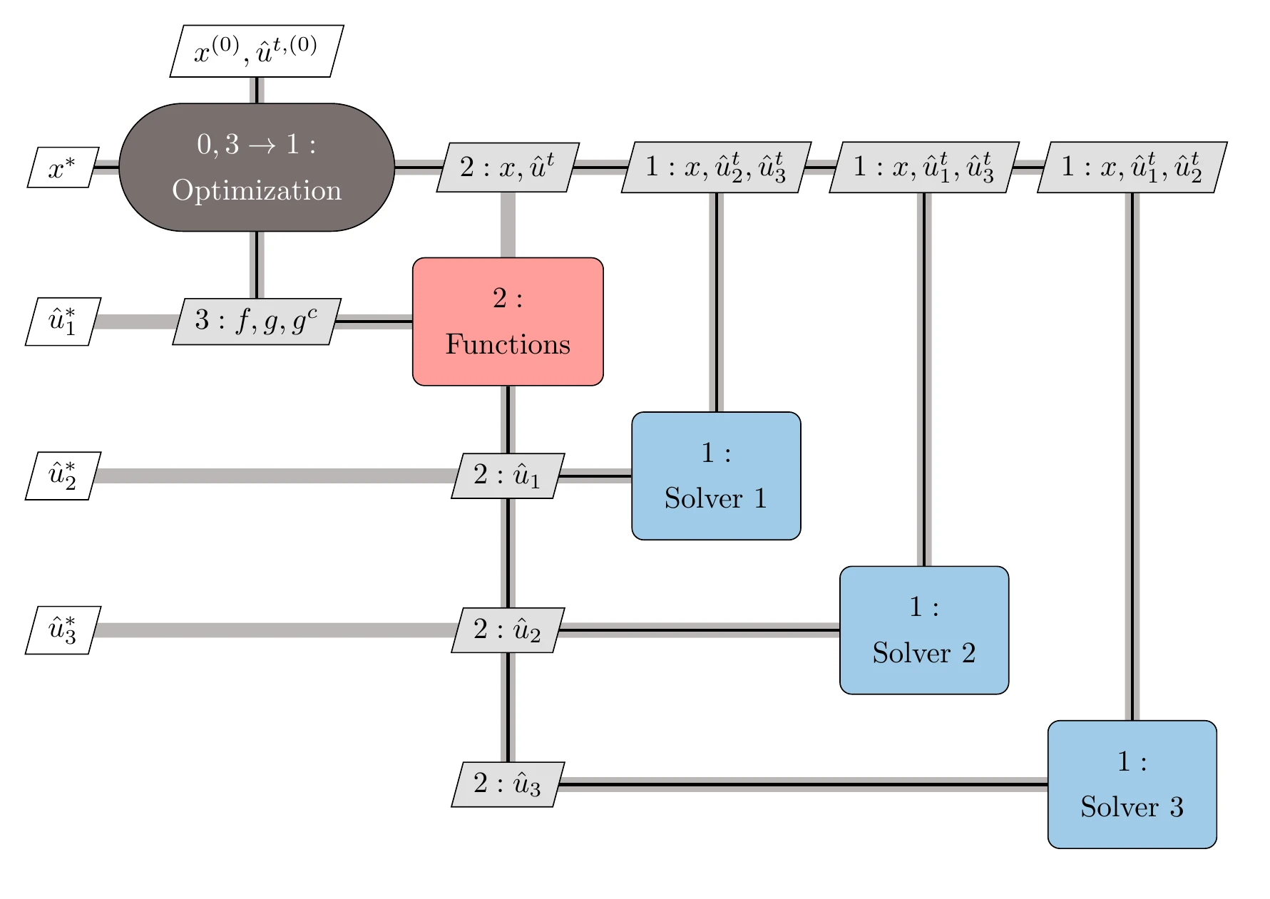
Figure 13.35:The IDF architecture breaks up the MDA by letting the optimizer solve for the coupling variables that satisfy interdisciplinary feasibility.
One advantage of IDF is that each component can be solved in parallel because they do not depend on each other directly. Another advantage is that if gradient-based optimization is used to solve the problem, the optimizer is typically more robust and has a better convergence rate than the fixed-point iteration algorithms of Section 13.2.5.
The main disadvantage of IDF is that the optimizer must handle more variables and constraints compared with the MDF architecture. If the number of coupling variables is large, the size of the resulting optimization problem may be too large to solve efficiently. This problem can be mitigated by careful selection of the components or by aggregating the coupling variables to reduce their dimensionality.
Unlike MDF, IDF does not guarantee a multidisciplinary feasible state at every design optimization iteration. Multidisciplinary feasibility is only guaranteed at the end of the optimization through the satisfaction of the consistency constraints. This is a disadvantage because if the optimization stops prematurely or we run out of time, we do not have a valid state for the coupled system.
13.4.3 Simultaneous Analysis and Design
Simultaneous analysis and design (SAND) extends the idea of IDF by moving not only the coupling variables to the optimization problem but also all component states. The SAND architecture requires exposing all the components in the form of the system-level view previously introduced in Figure 13.9. The residuals of the analysis become constraints for which the optimizer is responsible.[12]
This means that component solvers are no longer needed, and the optimizer becomes responsible for simultaneously solving the components for their states, the interdisciplinary compatibility for the coupling variables, and the design optimization problem for the design variables. All that is required from the model is the computation of residuals. Because the optimizer is controlling all these variables, SAND is also known as a full-space approach. SAND can be stated as follows:
Here, we use the representation shown in Figure 13.7, so there are two sets of explicit functions that convert the input coupling variables of the component. The SAND architecture is also applicable to single components, in which case there are no coupling variables. The XDSM for SAND is shown in Figure 13.36.
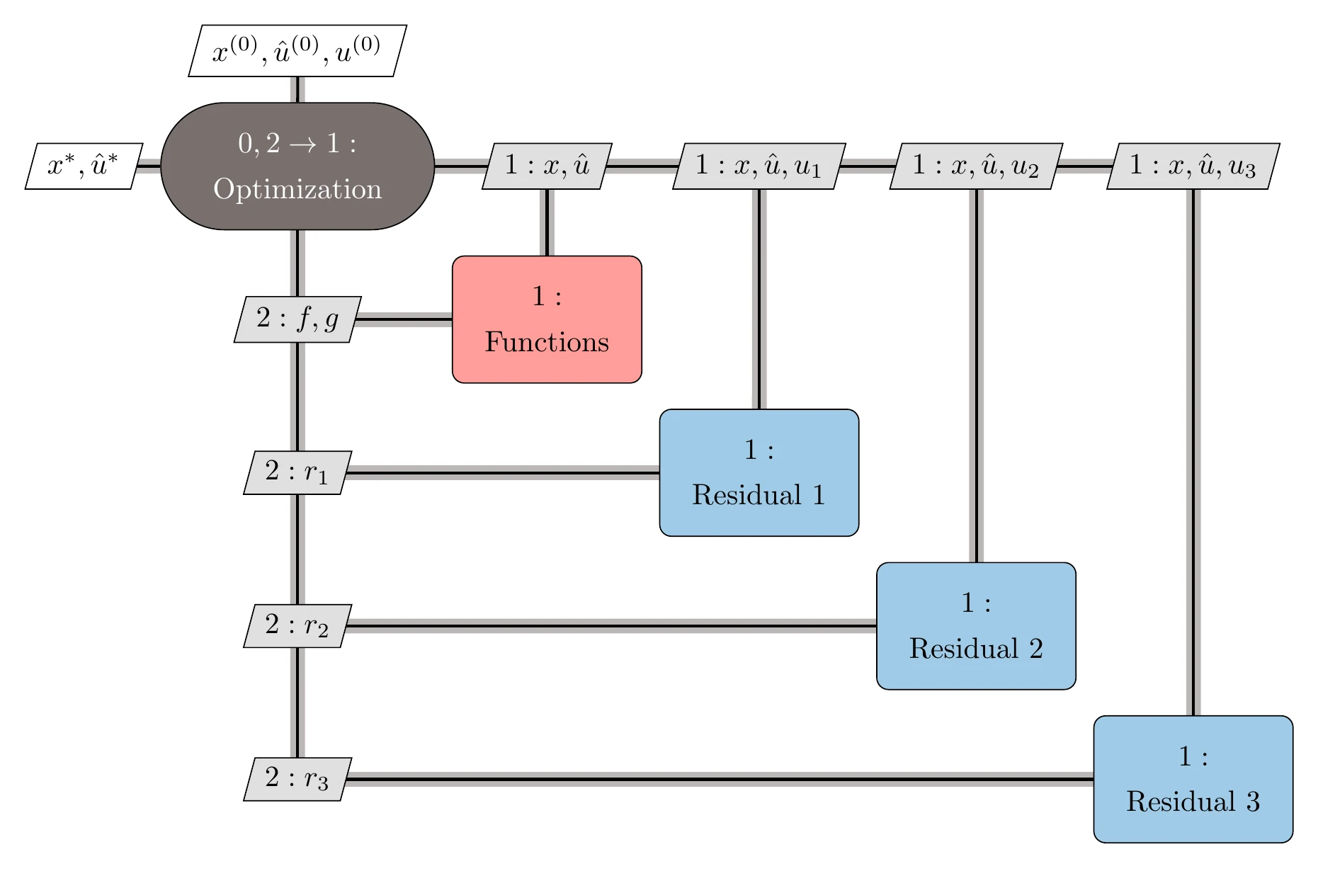
Figure 13.36:The SAND architecture lets the optimizer solve for all variables (design, coupling, and state variables), and component solvers are no longer needed.
Because it solves for all variables simultaneously, the SAND architecture can be the most efficient way to get to the optimal solution. In practice, however, it is unlikely that this is advantageous when efficient component solvers are available.
The resulting optimization problem is the largest of all MDO architectures and requires an optimizer that scales well with the number of variables. Therefore, a gradient-based optimization algorithm is likely required, in which case the derivative computation must also be considered. Fortunately, SAND does not require derivatives of the coupled system or even total derivatives that account for the component solution; only partial derivatives of residuals are needed.
SAND is an intrusive approach because it requires access to residuals. These might not be available if components are provided as black boxes. Rather than computing coupling variables and state variables by converging the residuals to zero, each component just computes the current residuals for the current values of the coupling variables and the component states .
13.5 Distributed MDO Architectures
The monolithic MDO architectures we have covered so far form and solve a single optimization problem. Distributed architectures decompose this single optimization problem into a set of smaller optimization problems, or disciplinary subproblems, which are then coordinated by a system-level subproblem. One key requirement for these architectures is that they must be mathematically equivalent to the original monolithic problem to converge to the same solution.
There are two primary motivations for distributed architectures. The first one is the possibility of decomposing the problem to reduce the computational time. The second motivation is to mimic the structure of large engineering design teams, where disciplinary groups have the autonomy to design their subsystems so that MDO is more readily adopted in industry. Overall, distributed MDO architectures have fallen short on both of these expectations. Unless a problem has a special structure, there is no distributed architecture that converges as rapidly as a monolithic one. In practice, distributed architectures have not been used much recently.
There are two main types of distributed architectures: those that enforce multidisciplinary feasibility via an MDA somewhere in the process and those that enforce multidisciplinary feasibility in some other way (using constraints or penalties at the system level). This is analogous to MDF and IDF, respectively, so we name these types distributed MDF and distributed IDF.[13]
In MDO problems, it can be helpful to distinguish between design variables that affect only one component directly (called local design variables) and design variables that affect two or more components directly (called shared design variables). We denote the vector of design variables local to component by and the shared variables by . The full vector of design variables is given by concatenating the shared and local design variables into a single vector , where is the number of components.
If a constraint can be computed using a single component and satisfied by varying only the local design variables for that component, it is a local constraint; otherwise, it is nonlocal. Similarly, for the design variables, we concatenate the constraints as . The same distinction could be applied to the objective function, but we do not usually do this.
The MDO problem representation we use here is shown in Figure 13.37 for a general three-component system. We use the functional form introduced in Section 13.2.3, where the states in each component are hidden. In this form, the system level only has access to the outputs of each solver, which are the coupling variables and functions of interest.
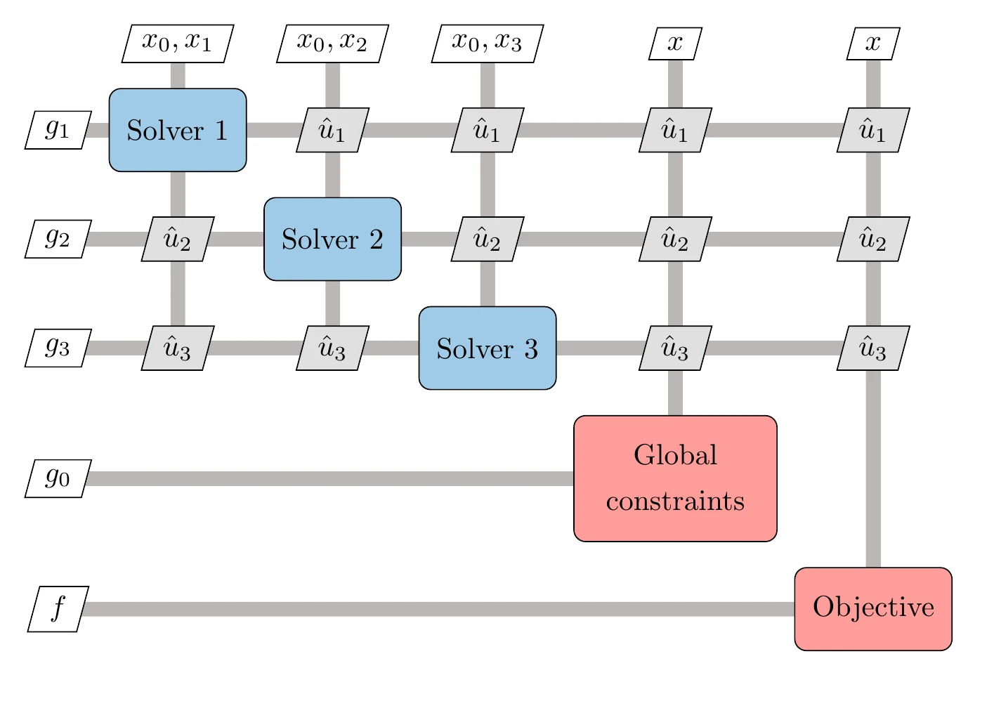
Figure 13.37:MDO problem nomenclature and dependencies.
The set of constraints is also split into shared constraints and local ones. Local constraints are computed by the corresponding component and depend only on the variables available in that component. Shared constraints depend on more than one set of coupling variables. These dependencies are also shown in Figure 13.37.
13.5.1 Collaborative Optimization
The collaborative optimization (CO) architecture is inspired by how disciplinary teams work to design complex engineered systems.14 This is a distributed IDF architecture, where the disciplinary optimization problems are formulated to be independent of each other by using target values of the coupling and shared design variables. These target values are then shared with all disciplines during every iteration of the solution procedure. The complete independence of disciplinary subproblems combined with the simplicity of the data-sharing protocol makes this architecture attractive for problems with a small amount of shared data.
The system-level subproblem modifies the original problem as follows: (1) local constraints are removed, (2) target coupling variables, , are added as design variables, and (3) a consistency constraint is added. This optimization problem can be written as follows:
where are copies of the shared design variables that are passed to discipline , and are copies of the local design variables passed to the system subproblem.
The constraint function is a measure of the inconsistency between the values requested by the system-level subproblem and the results from the discipline subproblem. The disciplinary subproblems do not include the original objective function. Instead, the objective of each subproblem is to minimize the inconsistency function.
For each discipline , the subproblem is as follows:
These subproblems are independent of each other and can be solved in parallel. Thus, the system-level subproblem is responsible for minimizing the design objective, whereas the discipline subproblems minimize system inconsistency while satisfying local constraints.
The CO problem statement has been shown to be mathematically equivalent to the original MDO problem.14 There are two versions of the CO architecture: CO and CO. Here, we only present the CO version. The XDSM for CO is shown in Figure 13.38 and the procedure is detailed in Algorithm 13.5.
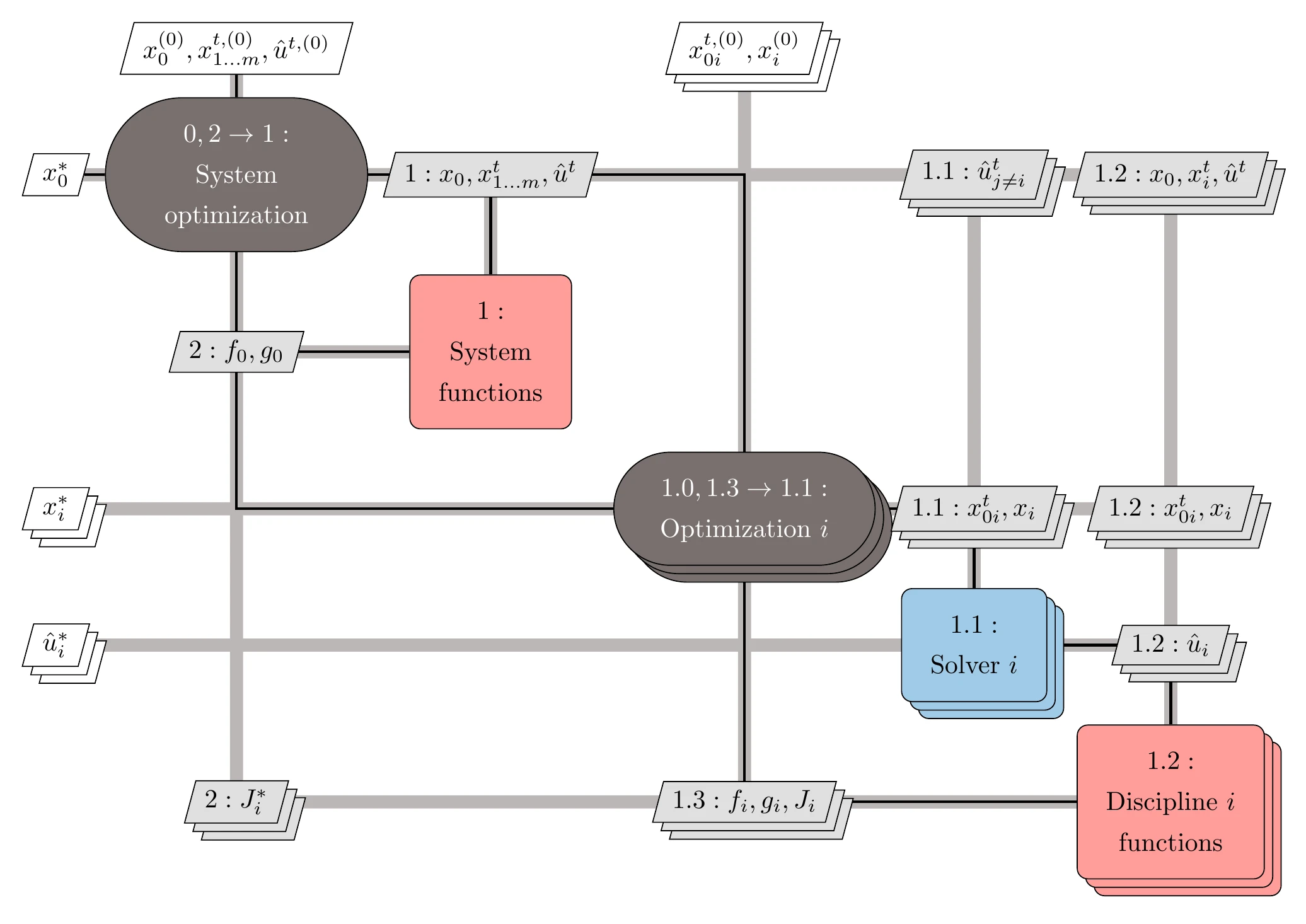
Figure 13.38:Diagram for the CO architecture.
CO has the organizational advantage of having entirely separate disciplinary subproblems. This is desirable when designers in each discipline want to maintain some autonomy. However, the CO formulation suffers from numerical ill-conditioning. This is because the constraint gradients of the system problem at an optimal solution are all zero vectors, which violates the constraint qualification requirement for the Karush–Kuhn–Tucker (KKT) conditions (see Section 5.3.1).
This ill-conditioning slows down convergence when using a gradient-based optimization algorithm or prevents convergence altogether.
13.5.2 Analytical Target Cascading
Analytical target cascading (ATC) is a distributed IDF architecture that uses penalties in the objective function to minimize the difference between the target variables requested by the system-level optimization and the actual variables computed by each discipline.[14]
The idea of ATC is similar to the CO architecture in the previous section, except that ATC uses penalties instead of a constraint. The ATC system-level problem is as follows:
where is a penalty relaxation of the shared design constraints, and is a penalty relaxation of the discipline consistency constraints.
Although the most common penalty functions in ATC are quadratic penalty functions, other penalty functions are possible. As mentioned in Section 5.4, penalty methods require a good selection of the penalty weight values to converge quickly and accurately enough. The ATC architecture converges to the same optimum as other MDO architectures, provided that problem is unimodal and all the penalty terms in the optimization problems approach zero.
Figure 13.39 shows the ATC architecture XDSM, where denotes the penalty function weights used in the determination of and . The details of ATC are described in Algorithm 13.6.
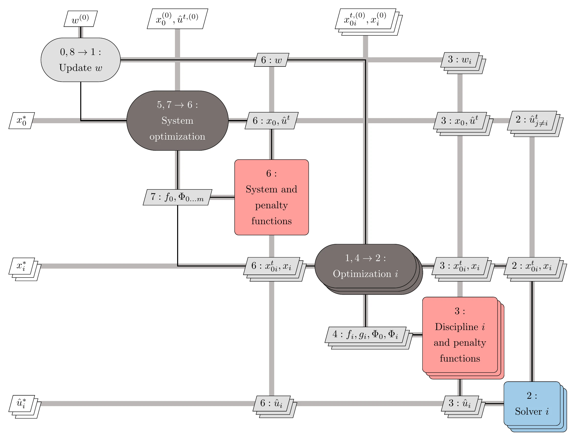
Figure 13.39:Diagram for the ATC architecture
The th discipline subproblem is as follows:
The most common penalty functions used in ATC are quadratic penalty functions (see Section 5.4.1). Appropriate penalty weights are important for multidisciplinary consistency and convergence.
13.5.3 Bilevel Integrated System Synthesis
Bilevel integrated system synthesis (BLISS) uses a series of linear approximations to the original design problem, with bounds on the design variable steps to prevent the design point from moving so far away that the approximations are too inaccurate.18 This is an idea similar to that of the trust-region methods in Section 4.5. These approximations are constructed at each iteration using coupled derivatives (see Section 13.3).
BLISS optimizes the local design variables within the discipline subproblems and the shared variables at the system level. The approach consists of using a series of linear approximations to the original optimization problem with limits on the design variable steps to stay within the region where the linear prediction yields the correct trend. This idea is similar to that of trust-region methods (see Section 4.5).
The system-level subproblem is formulated as follows:
The linearization is performed at each iteration using coupled derivative computation (see Section 13.3). The discipline subproblem is given by the following:
The extra set of constraints in both system-level and discipline subproblems denotes the design variable bounds.
To prevent violation of the disciplinary constraints by changes in the shared design variables, post-optimality derivatives are required to solve the system-level subproblem. In this case, the post-optimality derivatives quantify the change in the optimized disciplinary constraints with respect to a change in the system design variables, which can be estimated with the Lagrange multipliers of the active constraints (see Section 5.3.3 and Section 5.3.4).
Figure 13.40 shows the XDSM for BLISS, and the corresponding steps are listed in Algorithm 13.7. Because BLISS uses an MDA, it is a distributed MDF architecture. As a result of the linear nature of the optimization problems, repeated interrogation of the objective and constraint functions is not necessary once we have the gradients. If the underlying problem is highly nonlinear, the algorithm may converge slowly. The variable bounds may help the convergence if these bounds are properly chosen, such as through a trust-region framework.
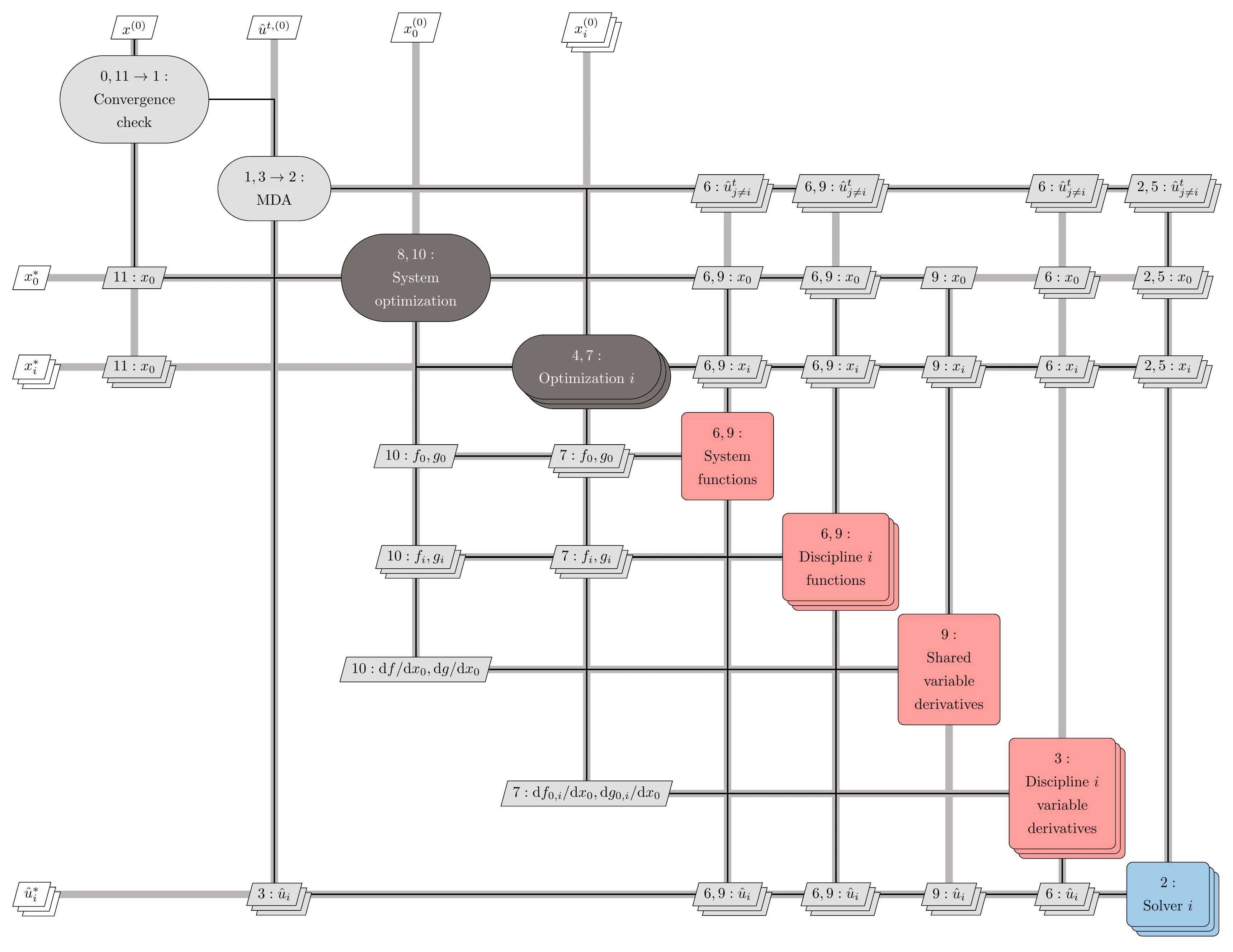
Figure 13.40:Diagram for the BLISS architecture.
13.5.4 Asymmetric Subspace Optimization
Asymmetric subspace optimization (ASO) is a distributed MDF architecture motivated by cases where there is a large discrepancy between the cost of the disciplinary solvers. The cheaper disciplinary analyses are replaced by disciplinary design optimizations inside the overall MDA to reduce the number of more expensive disciplinary analyses.
The system-level optimization subproblem is as follows:
The subscript denotes disciplinary information that remains outside of the MDA. The disciplinary optimization subproblem for discipline , which is resolved inside the MDA, is as follows:
Figure 13.41 shows a three-discipline case where the third discipline replaced with an optimization subproblem. ASO is detailed in Algorithm 13.8. To solve the system-level problem with a gradient-based optimizer, we require post-optimality derivatives of the objective and constraints with respect to the subproblem inputs (see Section 5.3.4).
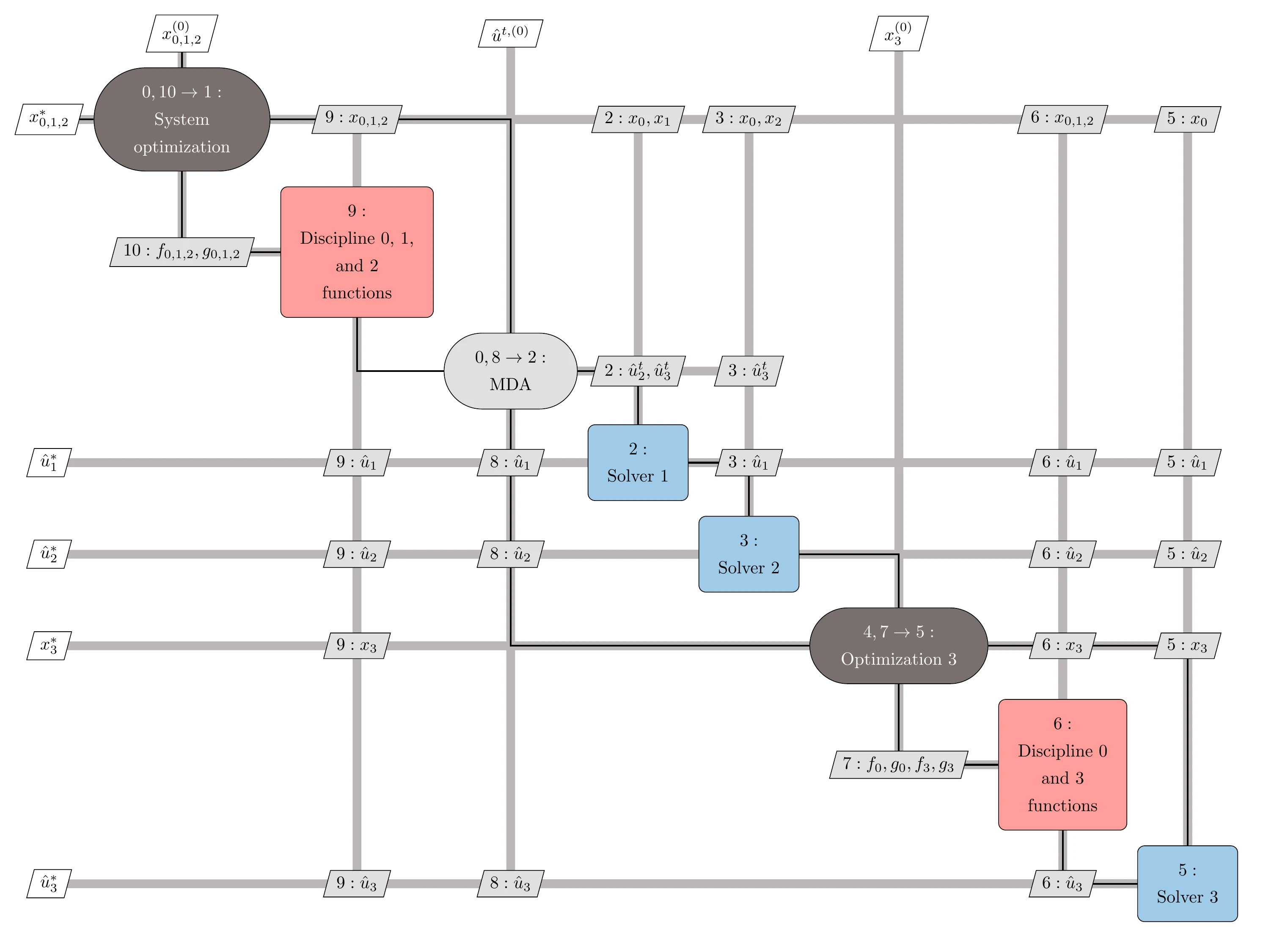
Figure 13.41:Diagram for the ASO architecture.
For a gradient-based system-level optimizer, the gradients of the objective and constraints must take into account the suboptimization. This requires coupled post-optimality derivative computation, which increases computational and implementation time costs compared with a normal coupled derivative computation. The total optimization cost is only competitive with MDF if the discrepancy between each disciplinary solver is high enough.
13.5.5 Other Distributed Architectures
There are other distributed MDF architectures in addition to BLISS and ASO: concurrent subspace optimization (CSSO) and MDO of independent subspaces (MDOIS).13
CSSO requires surrogate models for the analyses for all disciplines. The system-level optimization subproblem is solved based on the surrogate models and is therefore fast. The discipline-level optimization subproblem uses the actual analysis from the corresponding discipline and surrogate models for all other disciplines. The solutions for each discipline subproblem are used to update the surrogate models.
MDOIS only applies when no shared variables exist. In this case, discipline subproblems are solved independently, assuming fixed coupling variables, and then an MDA is performed to update the coupling.
There are also other distributed IDF architectures. Some of these are similar to CO in that they use a multilevel approach to enforce multidisciplinary feasibility: BLISS-2000 and quasi-separable decomposition (QSD). Other architectures enforce multidisciplinary feasibility with penalties, like ATC: inexact penalty decomposition (IPD), exact penalty decomposition (EPD), and enhanced collaborative optimization (ECO).
BLISS-2000 is a variation of BLISS that uses surrogate models to represent the coupling variables for all disciplines. Each discipline subproblem minimizes the linearized objective with respect to local variables subject to local constraints. The system-level subproblem minimizes the objective with respect to the shared variables and coupling variables while enforcing consistency constraints.
When using QSD, the objective and constraint functions are assumed to depend only on the shared design variables and coupling variables. Each discipline is assigned a “budget” for a local objective, and the discipline problems maximize the margin in their local constraints and the budgeted objective. The system-level subproblem minimizes the objective and budgets of each discipline while enforcing the shared constraints and a positive margin for each discipline.
IPD and EPD apply to MDO problems with no shared objectives or constraints. They are similar to ATC in that copies of the shared variables are used for every discipline subproblem, and the consistency constraints are relaxed with a penalty function. Unlike ATC, however, the more straightforward structure of the discipline subproblems is exploited to compute post-optimality derivatives to guide the system-level optimization subproblem.
Like CO, ECO uses copies of the shared variables. The discipline subproblems minimize quadratic approximations of the objective while enforcing local constraints and linear models of the nonlocal constraints. The system-level subproblem minimizes the total violation of all consistency constraints with respect to the shared variables.
13.6 Summary
MDO architectures provide different options for solving MDO problems. An acceptable MDO architecture must be mathematically equivalent to the original problem and converge to the same optima.
Sequential optimization, although intuitive, is not mathematically equivalent to the original problem and yields a design inferior to the MDO optimum.
MDO architectures are divided into two broad categories: monolithic architectures and distributed architectures. Monolithic architectures solve a single optimization problem, whereas distributed architectures solve optimization subproblems for each discipline and a system-level optimization problem. Overall, monolithic architectures exhibit a much better convergence rate than distributed architectures.19
In the last few years, the vast majority of MDO applications have used monolithic MDO architectures. The MAUD architecture, which can implement MDF, IDF, or a hybrid of the two, successfully solves large-scale MDO problems.8
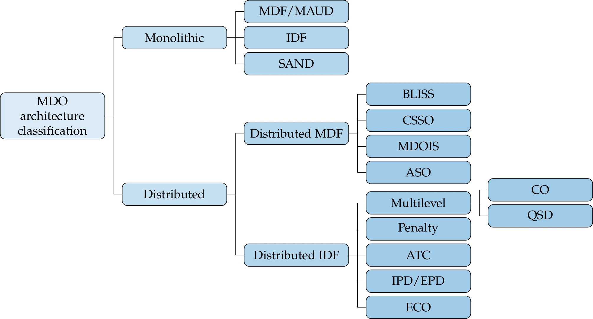
Figure 13.42:Classification of MDO architectures.
The distributed architectures can be divided according to whether or not they enforce multidisciplinary feasibility (through an MDA of the whole system), as shown in Figure 13.42. Distributed MDF architectures enforce multidisciplinary feasibility through an MDA. The distributed IDF architectures are like IDF in that no MDA is required. However, they must ensure multidisciplinary feasibility in some other way. Some do this by formulating an appropriate multilevel optimization (such as CO), and others use penalties to ensure this (such as ATC).[15]
Several commercial MDO frameworks are available, including Isight/SEE 20 by Dassault Systemes, ModelCenter/CenterLink by Phoenix Integration, modeFRONTIER by Esteco, AML Suite by TechnoSoft, Optimus by Noesis Solutions, and VisualDOC by Vanderplaats Research and Development.21 These frameworks focus on making it easy for users to couple multiple disciplines and use the optimization algorithms through graphical user interfaces. They also provide convenient wrappers to popular commercial engineering tools.
Typically, these frameworks use fixed-point iteration to converge the MDA. When derivatives are needed for a gradient-based optimizer, finite-difference approximations are used rather than more accurate analytic derivatives.
Problems
In some of the DSM literature, this definition is reversed, where “row” and “column” are interchanged, resulting in a transposed matrix.
Although these methods were designed for symmetric matrices, they are still useful for non-symmetric ones. Several numerical libraries include these methods.
In this chapter, we use a superscript for the iteration number instead of subscript to avoid a clash with the component index.
MAUD was developed by 9 when they realized that the unified derivatives equation (UDE) provides the mathematical foundation for a framework of parallel hierarchical solvers through a small set of user-defined functions. MAUD can also compute the derivatives of coupled systems, as we will see in Section 13.3.3.
As in Example 13.5, these results were obtained using OpenAeroStruct, and the description and equations are simplified for brevity.
The quantities after the semicolon in the variable dependence correspond to variables that remain fixed in the current context. For simplicity, we omit the design equality constraints () without loss of generality.
These are identical to the residuals of the system-level Newton solver (Equation 13.11).
- Jasa, J. P., Hwang, J. T., & Martins, J. R. R. A. (2018). Open-source coupled aerostructural optimization using Python. Structural and Multidisciplinary Optimization, 57(4), 1815–1827. 10.1007/s00158-018-1912-8
- Cuthill, E., & McKee, J. (1969). Reducing the bandwidth of sparse symmetric matrices. In Proceedings of the 1969 24th National Conference (pp. 157–172). Association for Computing Machinery. 10.1145/800195.805928
- Amestoy, P. R., Davis, T. A., & Duff, I. S. (1996). An approximate minimum degree ordering algorithm. SIAM Journal on Matrix Analysis and Applications, 17(4), 886–905. 10.1137/S0895479894278952
- Lambe, A. B., & Martins, J. R. R. A. (2012). Extensions to the design structure matrix for the description of multidisciplinary design, analysis, and optimization processes. Structural and Multidisciplinary Optimization, 46, 273–284. 10.1007/s00158-012-0763-y
- Irons, B. M., & Tuck, R. C. (1969). A version of the Aitken accelerator for computer iteration. International Journal for Numerical Methods in Engineering, 1(3), 275–277. 10.1002/nme.1620010306
- Kenway, G. K. W., Kennedy, G. J., & Martins, J. R. R. A. (2014). Scalable parallel approach for high-fidelity steady-state aeroelastic analysis and derivative computations. AIAA Journal, 52(5), 935–951. 10.2514/1.J052255
- Chauhan, S. S., Hwang, J. T., & Martins, J. R. R. A. (2018). An automated selection algorithm for nonlinear solvers in MDO. Structural and Multidisciplinary Optimization, 58(2), 349–377. 10.1007/s00158-018-2004-5
- Gray, J. S., Hwang, J. T., Martins, J. R. R. A., Moore, K. T., & Naylor, B. A. (2019). OpenMDAO: An open-source framework for multidisciplinary design, analysis, and optimization. Structural and Multidisciplinary Optimization, 59(4), 1075–1104. 10.1007/s00158-019-02211-z
- Hwang, J. T., & Martins, J. R. R. A. (2018). A computational architecture for coupling heterogeneous numerical models and computing coupled derivatives. ACM Transactions on Mathematical Software, 44(4), Article 37. 10.1145/3182393
- Kenway, G. K. W., & Martins, J. R. R. A. (2014). Multipoint high-fidelity aerostructural optimization of a transport aircraft configuration. Journal of Aircraft, 51(1), 144–160. 10.2514/1.C032150
- Hwang, J. T., Lee, D. Y., Cutler, J. W., & Martins, J. R. R. A. (2014). Large-scale multidisciplinary optimization of a small satellite’s design and operation. Journal of Spacecraft and Rockets, 51(5), 1648–1663. 10.2514/1.A32751
- Biegler, L. T., Ghattas, O., Heinkenschloss, M., & van Bloemen Waanders, B. (Eds.). (2003). Large-Scale PDE-Constrained Optimization. Springer. https://www.google.ca/books/edition/Large_Scale_PDE_Constrained_Optimization/O4YKBwAAQBAJ
- Martins, J. R. R. A., & Lambe, A. B. (2013). Multidisciplinary design optimization: A survey of architectures. AIAA Journal, 51(9), 2049–2075. 10.2514/1.J051895
- Braun, R. D., & Kroo, I. M. (1997). Development and application of the collaborative optimization architecture in a multidisciplinary design environment. In N. Alexandrov & M. Y. Hussaini (Eds.), Multidisciplinary Design Optimization: State of the Art (pp. 98–116). SIAM. 10.5555/888020
- Kim, H. M., Rideout, D. G., Papalambros, P. Y., & Stein, J. L. (2003). Analytical target cascading in automotive vehicle design. Journal of Mechanical Design, 125(3), 481–490. 10.1115/1.1586308