1 Introduction
Optimization is a human instinct. People constantly seek to improve their lives and the systems that surround them. Optimization is intrinsic in biology, as exemplified by the evolution of species. Birds optimize their wings’ shape in real time, and dogs have been shown to find optimal trajectories. Even more broadly, many laws of physics relate to optimization, such as the principle of minimum energy. As Leonhard Euler once wrote, “nothing at all takes place in the universe in which some rule of maximum or minimum does not appear.”
The term optimization is often used to mean “improvement”, but mathematically, it is a much more precise concept: finding the best possible solution by changing variables that can be controlled, often subject to constraints. Optimization has a broad appeal because it is applicable in all domains and because of the human desire to make things better. Any problem where a decision needs to be made can be cast as an optimization problem.
Although some simple optimization problems can be solved analytically, most practical problems of interest are too complex to be solved this way. The advent of numerical computing, together with the development of optimization algorithms, has enabled us to solve problems of increasing complexity.
Optimization problems occur in various areas, such as economics, political science, management, manufacturing, biology, physics, and engineering. This book focuses on the application of numerical optimization to the design of engineering systems. Numerical optimization first emerged in operations research, which deals with problems such as deciding on the price of a product, setting up a distribution network, scheduling, or suggesting routes. Other optimization areas include optimal control and machine learning. Although we do not cover these other areas specifically in this book, many of the methods we cover are useful in those areas.
Design optimization problems abound in the various engineering disciplines, such as wing design in aerospace engineering, process control in chemical engineering, structural design in civil engineering, circuit design in electrical engineering, and mechanism design in mechanical engineering. Most engineering systems rarely work in isolation and are linked to other systems. This gave rise to the field of multidisciplinary design optimization (MDO), which applies numerical optimization techniques to the design of engineering systems that involve multiple disciplines.
In the remainder of this chapter, we start by explaining the design optimization process and contrasting it with the conventional design process (Section 1.1). Then we explain how to formulate optimization problems and the different types of problems that can arise (Section 1.2). Because design optimization problems involve functions of different types, these are also briefly discussed (Section 1.3). (A more detailed discussion of the numerical models used to compute these functions is deferred to Chapter 3.) We then provide an overview of the different optimization algorithms, highlighting the algorithms covered in this book and linking to the relevant sections (Section 1.4). We connect algorithm types and problem types by providing guidelines for selecting the right algorithm for a given problem (Section 1.5). Finally, we introduce the notation used throughout the book (Section 1.6).
1.1 Design Optimization Process
Engineering design is an iterative process that engineers follow to develop a product that accomplishes a given task. For any product beyond a certain complexity, this process involves teams of engineers and multiple stages with many iterative loops that may be nested. The engineering teams are formed to tackle different aspects of the product at different stages.
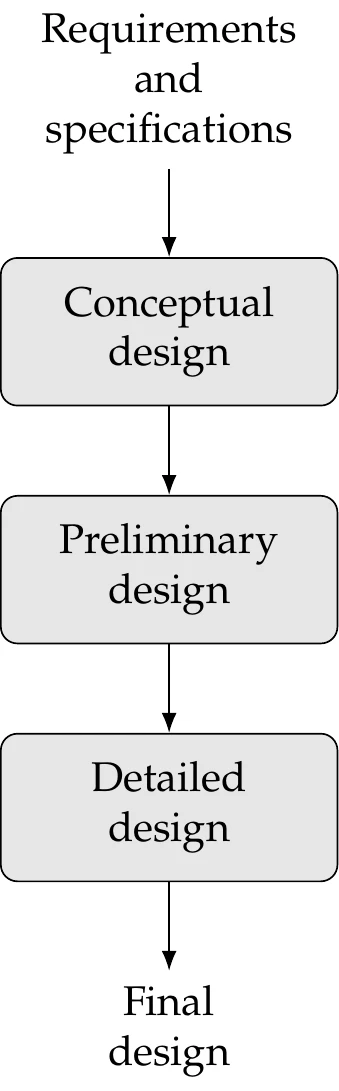
Figure 1.1:Design phases.
The design process can be divided into the sequence of phases shown in Figure 1.1. Before the design process begins, we must determine the requirements and specifications. This might involve market research, an analysis of current similar designs, and interviews with potential customers.
In the conceptual design phase, various concepts for the system are generated and considered. Because this phase should be short, it usually relies on simplified models and human intuition. For more complicated systems, the various subsystems are identified. In the preliminary design phase, a chosen concept and subsystems are refined by using better models to guide changes in the design, and the performance expectations are set. The detailed design phase seeks to complete the design down to every detail so that it can finally be manufactured. All of these phases require iteration within themselves. When severe issues are identified, it may be necessary to “go back to the drawing board” and regress to an earlier phase. This is just a high-level view; in practical design, each phase may require multiple iterative processes.
Design optimization is a tool that can replace an iterative design process to accelerate the design cycle and obtain better results. To understand the role of design optimization, consider a simplified version of the conventional engineering design process with only one iterative loop, as shown in Figure 1.2 (top). In this process, engineers make decisions at every stage based on intuition and background knowledge.
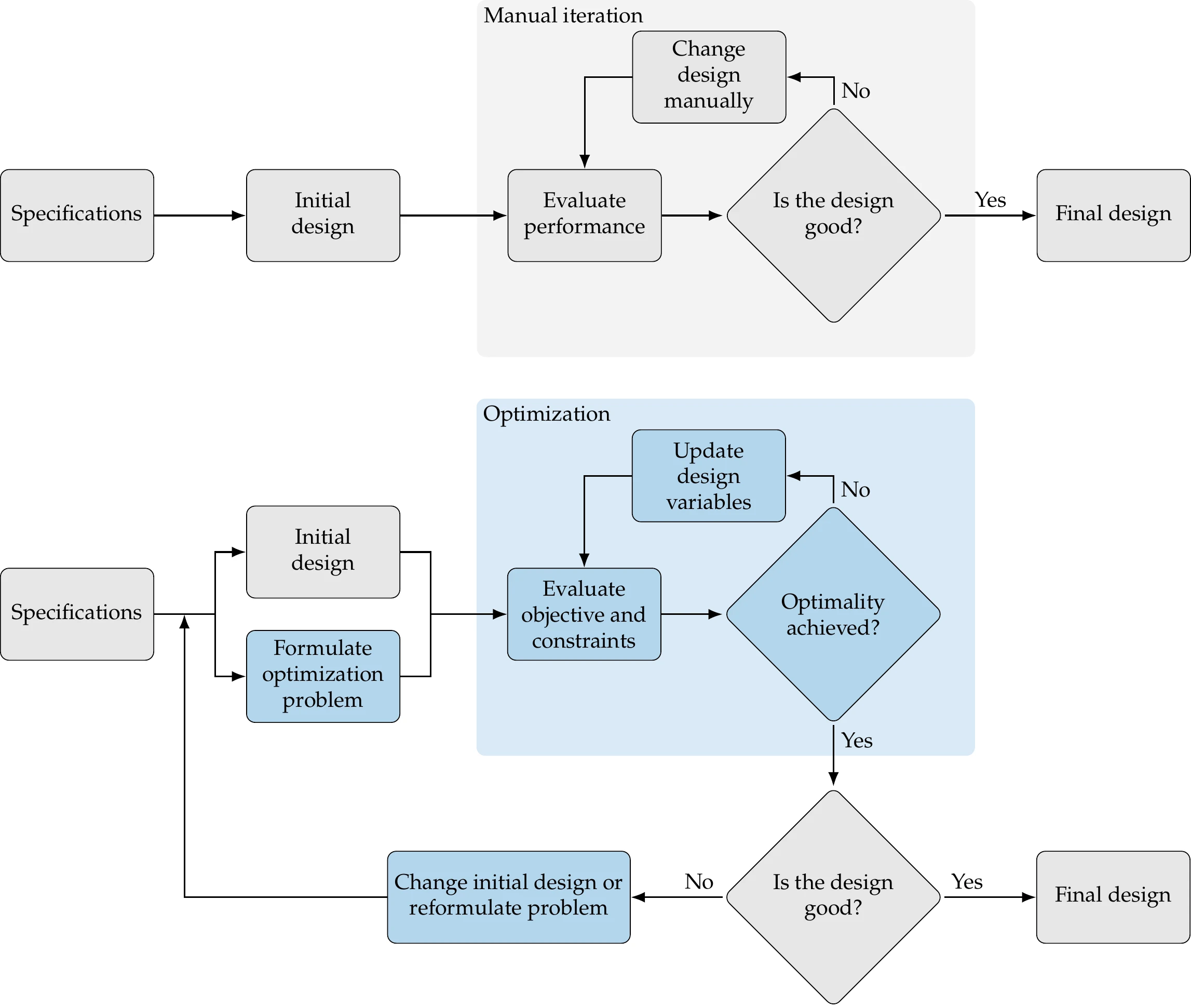
Figure 1.2:Conventional (top) versus design optimization process (bottom).
Each of the steps in the conventional design process includes human decisions that are either challenging or impossible to program into computer code. Determining the product specifications requires engineers to define the problem and do background research. The design cycle must start with an initial design, which can be based on past designs or a new idea. In the conventional design process, this initial design is analyzed in some way to evaluate its performance. This could involve numerical modeling or actual building and testing. Engineers then evaluate the design and decide whether it is good enough or not based on the results.[1] If the answer is no—which is likely to be the case for at least the first few iterations—the engineer changes the design based on intuition, experience, or trade studies. When the design is finalized when it is deemed satisfactory.
The design optimization process can be represented using a flow diagram similar to that for the conventional design process, as shown in Figure 1.2 (bottom). The determination of the specifications and the initial design are no different from the conventional design process. However, design optimization requires a formal formulation of the optimization problem that includes the design variables that are to be changed, the objective to be minimized, and the constraints that need to be satisfied. The evaluation of the design is strictly based on numerical values for the objective and constraints. When a rigorous optimization algorithm is used, the decision to finalize the design is made only when the current design satisfies the optimality conditions that ensure that no other design “close by” is better. The design changes are made automatically by the optimization algorithm and do not require intervention from the designer.
This automated process does not usually provide a “push-button” solution; it requires human intervention and expertise (often more expertise than in the traditional process). Human decisions are still needed in the design optimization process. Before running an optimization, in addition to determining the specifications and initial design, engineers need to formulate the design problem. This requires expertise in both the subject area and numerical optimization. The designer must decide what the objective is, which parameters can be changed, and which constraints must be enforced. These decisions have profound effects on the outcome, so it is crucial that the designer formulates the optimization problem well.
After running the optimization, engineers must assess the design because it is unlikely that the first formulation yields a valid and practical design. After evaluating the optimal design, engineers might decide to reformulate the optimization problem by changing the objective function, adding or removing constraints, or changing the set of design variables. Engineers might also decide to increase the models’ fidelity if they fail to consider critical physical phenomena, or they might decide to decrease the fidelity if the models are too expensive to evaluate in an optimization iteration.
Post-optimality studies are often performed to interpret the optimal design and the design trends. This might be done by performing parameter studies, where design variables or other parameters are varied to quantify their effect on the objective and constraints. Validation of the result can be done by evaluating the design with higher-fidelity simulation tools, by performing experiments, or both. It is also possible to compute post-optimality sensitivities to evaluate which design variables are the most influential or which constraints drive the design. These sensitivities can inform where engineers might best allocate resources to alleviate the driving constraints in future designs.
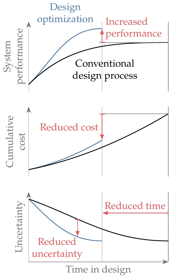
Figure 1.3:Compared with the conventional design process, MDO increases the system performance, decreases the design time, reduces the total cost, and reduces the uncertainty at a given point in time.
Design optimization can be used in any of the design phases shown in Figure 1.1, where each phase could involve running one or more design optimizations. We illustrate several advantages of design optimization in Figure 1.3, which shows the notional variations of system performance, cost, and uncertainty as a function of time in design. When using optimization, the system performance increases more rapidly compared with the conventional process, achieving a better end result in a shorter total time. As a result, the cost of the design process is lower. Finally, the uncertainty in the performance reduces more rapidly as well.
Considering multiple disciplines or components using MDO amplifies the advantages illustrated in Figure 1.3. The central idea of MDO is to consider the interactions between components using coupled models while simultaneously optimizing the design variables from the various components. In contrast, sequential optimization optimizes one component at a time. Even when interactions are considered, sequential optimization might converge to a suboptimal result (see Section 13.1 for more details and examples).
In this book, we tend to frame problems and discussions in the context of engineering design. However, the optimization methods are general and are used in other applications that may not be design problems, such as optimal control, machine learning, and regression. In other words, we mean “design” in a general sense, where variables are changed to optimize an objective.
1.2 Optimization Problem Formulation
The design optimization process requires the designer to translate their intent to a mathematical statement that can then be solved by an optimization algorithm. Developing this statement has the added benefit that it helps the designer better understand the problem. Being methodical in the formulation of the optimization problem is vital because the optimizer tends to exploit any weaknesses you might have in your formulation or model. An inadequate problem formulation can either cause the optimization to fail or cause it to converge to a mathematical optimum that is undesirable or unrealistic from an engineering point of view—the proverbial “right answer to the wrong question”.
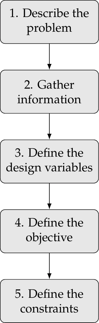
Figure 1.4:Steps in optimization problem formulation.
To formulate design optimization problems, we follow the procedure outlined in Figure 1.4.
The first step requires writing a description of the design problem, including a description of the system, and a statement of all the goals and requirements. At this point, the description does not necessarily involve optimization concepts and is often vague.
The next step is to gather as much data and information as possible about the problem. Some information is already specified in the problem statement, but more research is usually required to find all the relevant data on the performance requirements and expectations. Raw data might need to be processed and organized to gather the information required for the design problem. The more familiar practitioners are with the problem, the better prepared they will be to develop a sound formulation to identify eventual issues in the solutions.
At this stage, it is also essential to identify the analysis procedure and gather information on that as well. The analysis might consist of a simple model or a set of elaborate tools. All the possible inputs and outputs of the analysis should be identified, and its limitations should be understood. The computational time for the analysis needs to be considered because optimization requires repeated analysis.
It is usually impossible to learn everything about the problem before proceeding to the next steps, where we define the design variables, objective, and constraints. Therefore, information gathering and refinement are ongoing processes in problem formulation.
1.2.1 Design Variables
The next step is to identify the variables that describe the system, the design variables,[2]which we represent by the column vector:
This vector defines a given design, so different vectors correspond to different designs. The number of variables, , determines the problem’s dimensionality.
The design variables must not depend on each other or any other parameter, and the optimizer must be free to choose the elements of independently. This means that in the analysis of a given design, the variables must be input parameters that remain fixed throughout the analysis process. Otherwise, the optimizer does not have absolute control of the design variables. Another possible pitfall is to define a design variable that happens to be a linear combination of other variables, which results in an ill-defined optimization problem with an infinite number of combinations of design variable values that correspond to the same design.
The choice of variables is usually not unique. For example, a square shape can be parametrized by the length of its side or by its area, and different unit systems can be used. The choice of units affects the problem’s scaling but not the functional form of the problem.
The choice of design variables can affect the functional form of the objective and constraints. For example, some nonlinear relationships can be converted to linear ones through a change of variables. It is also possible to introduce or eliminate discontinuities through the choice of design variables.
A given set of design variable values defines the system’s design, but whether this system satisfies all the requirements is a separate question that will be addressed with the constraints in a later step. However, it is possible and advisable to define the space of allowable values for the design variables based on the design problem’s specifications and physical limitations.
The first consideration in the definition of the allowable design variable values is whether the design variables are continuous or discrete. Continuous design variables are real numbers that are allowed to vary continuously within a specified range with no gaps, which we write as
where and are lower and upper bounds on the design variables, respectively. These are also known as bound constraints or side constraints. Some design variables may be unbounded or bounded on only one side.
When all the design variables are continuous, the optimization problem is said to be continuous.[3]Most of this book focuses on algorithms that assume continuous design variables.
When one or more variables are allowed to have discrete values, whether real or integer, we have a discrete optimization problem. An example of a discrete design variable is structural sizing, where only components of specific thicknesses or cross-sectional areas are available. Integer design variables are a special case of discrete variables where the values are integers, such as the number of wheels on a vehicle. Optimization algorithms that handle discrete variables are discussed in Chapter 8.
We distinguish the design variable bounds from constraints because the optimizer has direct control over their values, and they benefit from a different numerical treatment when solving an optimization problem. When defining these bounds, we must take care not to unnecessarily constrain the design space, which would prevent the optimizer from achieving a better design that is realizable. A smaller allowable range in the design variable values should make the optimization easier. However, design variable bounds should be based on actual physical constraints instead of being artificially limited. An example of a physical constraint is a lower bound on structural thickness in a weight minimization problem, where otherwise, the optimizer will discover that negative sizes yield negative weight. Whenever a design variable converges to the bound at the optimum, the designer should reconsider the reasoning for that bound and make sure it is valid. This is because designers sometimes set bounds that limit the optimization from obtaining a better objective.
At the formulation stage, we should strive to list as many independent design variables as possible. However, it is advisable to start with a small set of variables when solving a problem for the first time and then gradually expand the set of design variables.
Some optimization algorithms require the user to provide initial design variable values. This initial point is usually based on the best guess the user can produce. This might be an already good design that the optimization refines further by making small changes. Another possibility is that the initial guess is a bad design or a “blank slate” that the optimization changes significantly.
1.2.2 Objective Function
To find the best design, we need an objective function, which is a quantity that determines if one design is better than another. This function must be a scalar that is computable for a given design variable vector . The objective function can be minimized or maximized, depending on the problem. For example, a designer might want to minimize the weight or cost of a given structure. An example of a function to be maximized could be the range of a vehicle.
The convention adopted in this book is that the objective function, , is to be minimized. This convention does not prevent us from maximizing a function because we can reformulate it as a minimization problem by finding the minimum of the negative of and then changing the sign, as follows:
This transformation is illustrated in Figure 1.8.[4]
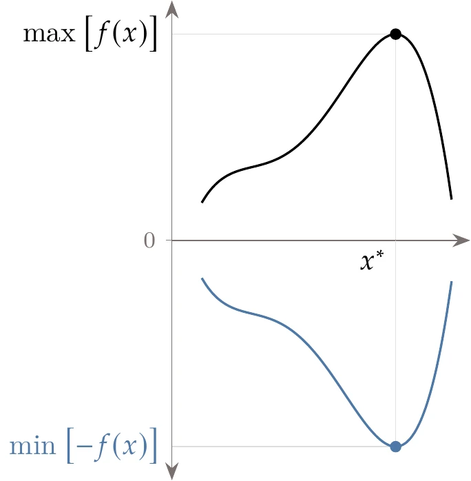
Figure 1.8:A maximization problem can be transformed into an equivalent minimization problem.
The objective function is computed through a numerical model whose complexity can range from a simple explicit equation to a system of coupled implicit models (more on this in Chapter 3).
The choice of objective function is crucial for successful design optimization. If the function does not represent the true intent of the designer, it does not matter how precisely the function and its optimum point are computed—the mathematical optimum will be non-optimal from the engineering point of view. A bad choice for the objective function is a common mistake in design optimization.
The choice of objective function is not always obvious. For example, minimizing the weight of a vehicle might sound like a good idea, but this might result in a vehicle that is too expensive to manufacture. In this case, manufacturing cost would probably be a better objective. However, there is a trade-off between manufacturing cost and the performance of the vehicle. It might not be obvious which of these objectives is the most appropriate one because this trade-off depends on customer preferences. This issue motivates multiobjective optimization, which is the subject of Chapter 9. Multiobjective optimization does not yield a single design but rather a range of designs that settle for different trade-offs between the objectives.
Experimenting with different objectives should be part of the design exploration process (this is represented by the outer loop in the design optimization process in Figure 1.2). Results from optimizing the “wrong” objective can still yield insights into the design trade-offs and trends for the system at hand.
In Example 1.1, we have the luxury of being able to visualize the design space because we have only two variables. For more than three variables, it becomes impossible to visualize the design space. We can also visualize the objective function for two variables, as shown in Figure 1.9. In this figure, we plot the function values using the vertical axis, which results in a three-dimensional surface. Although plotting the surface might provide intuition about the function, it is not possible to locate the points accurately when drawing on a two-dimensional surface.
Another possibility is to plot the contours of the function, which are lines of constant value, as shown in Figure 1.10.
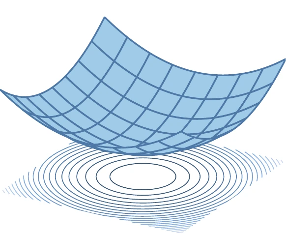
Figure 1.9:A function of two variables ( in this case) can be visualized by plotting a three-dimensional surface or contour plot.
We prefer this type of plot and use it extensively throughout this book because we can locate points accurately and get the correct proportions in the axes (in Figure 1.10, the contours are perfect circles, and the location of the minimum is clear). Our convention is to represent lower function values with darker lines and higher values with lighter ones.
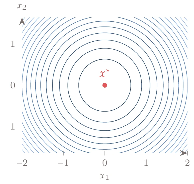
Figure 1.10:Contour plot of .
Unless otherwise stated, the function variation between two adjacent lines is constant, and therefore, the closer together the contour lines are, the faster the function is changing. The equivalent of a contour line in -dimensional space is a hypersurface of constant value with dimensions of , called an isosurface.
We use mostly two-dimensional examples throughout the book because we can visualize them conveniently. Such visualizations should give you an intuition about the methods and problems. However, keep in mind that general problems have many more dimensions, and only mathematics can help you in such cases.
Although we can sometimes visualize the variation of the objective function in a contour plot as in Example 1.2, this is not possible for problems with more design variables or more computationally demanding function evaluations. This motivates numerical optimization algorithms, which aim to find the minimum in a multidimensional design space using as few function evaluations as possible.
1.2.3 Constraints
The vast majority of practical design optimization problems require the enforcement of constraints. These are functions of the design variables that we want to restrict in some way. Like the objective function, constraints are computed through a model whose complexity can vary widely. The feasible region is the set of points that satisfy all constraints. We seek to minimize the objective function within this feasible design space.
When we restrict a function to being equal to a fixed value, we call this an equality constraint, denoted by . When the function is required to be less than or equal to a certain value, we have an inequality constraint, denoted by .[6] Although we use the “less or equal” convention, some texts and software programs use “greater or equal” instead. There is no loss of generality with either convention because we can always multiply the constraint by -1 to convert between the two.
Some texts and papers omit the equality constraints without loss of generality because an equality constraint can be replaced by two inequality constraints. More specifically, an equality constraint, , is equivalent to enforcing two inequality constraints, and .
Inequality constraints can be active or inactive at the optimum point. An active inequality constraint means that , whereas for an inactive one, . If a constraint is inactive at the optimum, this constraint could have been removed from the problem with no change in its solution, as illustrated in Figure 1.12. In this case, constraints and can be removed without affecting the solution of the problem. Furthermore, active constraints ( in this case) can equivalently be replaced by equality constraints. However, it is difficult to know in advance which constraints are active or not at the optimum for a general problem. Constrained optimization is the subject of Chapter 5.
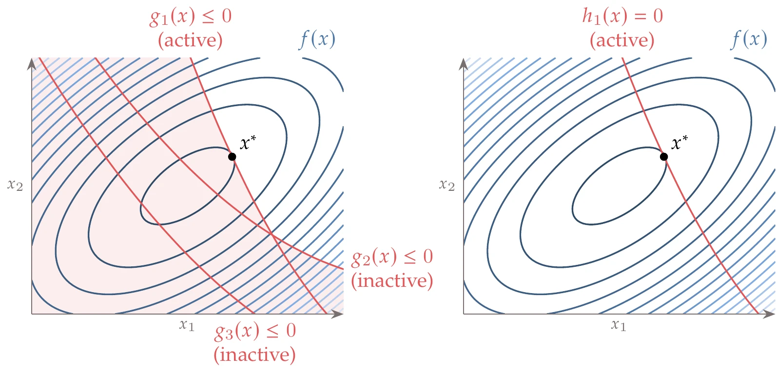
Figure 1.12:Two-dimensional problem with one active and two inactive inequality constraints (left). The shaded area indicates regions that are infeasible (i.e., the constraints are violated). If we only had the active single equality constraint in the formulation, we would obtain the same result (right).
It is possible to overconstrain the problem such that there is no solution. This can happen as a result of a programming error but can also occur at the problem formulation stage. For more complicated design problems, it might not be possible to satisfy all the specified constraints, even if they seem to make sense. When this happens, constraints have to be relaxed or removed.
The problem must not be overconstrained, or else there is no feasible region in the design space over which the function can be minimized. Thus, the number of independent equality constraints must be less than or equal to the number of design variables (). There is no limit on the number of inequality constraints. However, they must be such that there is a feasible region, and the number of active constraints plus the equality constraints must still be less than or equal to the number of design variables.
The feasible region grows when constraints are removed and shrinks when constraints are added (unless these constraints are redundant). As the feasible region grows, the optimum objective function usually improves or at least stays the same. Conversely, the optimum worsens or stays the same when the feasible region shrinks.
One common issue in optimization problem formulation is distinguishing objectives from constraints. For example, we might be tempted to minimize the stress in a structure, but this would inevitably result in an overdesigned, heavy structure. Instead, we might want minimum weight (or cost) with sufficient safety factors on stress, which can be enforced by an inequality constraint.
Most engineering problems require constraints—often a large number of them. Although constraints may at first appear limiting, they enable the optimizer to find useful solutions.
As previously mentioned, some algorithms require the user to provide an initial guess for the design variable values. Although it is easy to assign values within the bounds, it might not be as easy to ensure that the initial design satisfies the constraints. This is not an issue for most optimization algorithms, but some require starting with a feasible design.
As previously mentioned, it is generally not possible to visualize the design space as shown in Example 1.2 and obtain the solution graphically. In addition to the possibility of a large number of design variables and computationally expensive objective function evaluations, we now add the possibility of a large number of constraints, which might also be expensive to evaluate. Again, this is further motivation for the optimization techniques covered in this book.
1.2.4 Optimization Problem Statement
Now that we have discussed the design variables, the objective function, and constraints, we can put them all together in an optimization problem statement. In words, this statement is as follows: minimize the objective function by varying the design variables within their bounds subject to the constraints.
Mathematically, we write this statement as follows:
This is the standard formulation used in this book; however, other books and software manuals might differ from this.[7]For example, they might use different symbols, use “greater than or equal to” for the inequality constraint, or maximize instead of minimizing. In any case, it is possible to convert between standard formulations to get equivalent problems.
All continuous optimization problems with a single-objective can be written in the standard form shown in Equation 1.4. Although our target applications are engineering design problems, many other problems can be stated in this form, and thus, the methods covered in this book can be used to solve those problems.
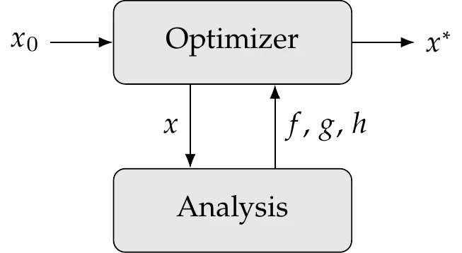
Figure 1.14:The analysis computes the objective () and constraint values (, ) for a given set of design variables ().
The values of the objective and constraint functions for a given set of design variables are computed through the analysis, which consists of one or more numerical models. The analysis must be fully automatic so that multiple optimization cycles can be completed without human intervention, as shown in Figure 1.14. The optimizer usually requires an initial design and then queries the analysis for a sequence of designs until it finds the optimum design, .
When the optimizer queries the analysis for a given , for most methods, the constraints do not have to be feasible. The optimizer is responsible for changing so that the constraints are satisfied.
The objective and constraint functions must depend on the design variables; if a function does not depend on any variable in the whole domain, it can be ignored and should not appear in the problem statement.
Ideally, , , and should be computable for all values of that make physical sense. Lower and upper design variable bounds should be set to avoid nonphysical designs as much as possible. Even after taking this precaution, models in the analysis sometimes fail to provide a solution. A good optimizer can handle such eventualities gracefully.
There are some mathematical transformations that do not change the solution of the optimization problem (Equation 1.4). Multiplying either the objective or the constraints by a constant does not change the optimal design; it only changes the optimum objective value. Adding a constant to the objective does not change the solution, but adding a constant to any constraint changes the feasible space and can change the optimal design.
Determining an appropriate set of design variables, objective, and constraints is a crucial aspect of the outer loop shown in Figure 1.2, which requires human expertise in engineering design and numerical optimization.
1.3 Optimization Problem Classification
To choose the most appropriate optimization algorithm for solving a given optimization problem, we must classify the optimization problem and know how its attributes affect the efficacy and suitability of the available optimization algorithms. This is important because no optimization algorithm is efficient or even appropriate for all types of problems.
We classify optimization problems based on two main aspects: the problem formulation and the characteristics of the objective and constraint functions, as shown in Figure 1.15.
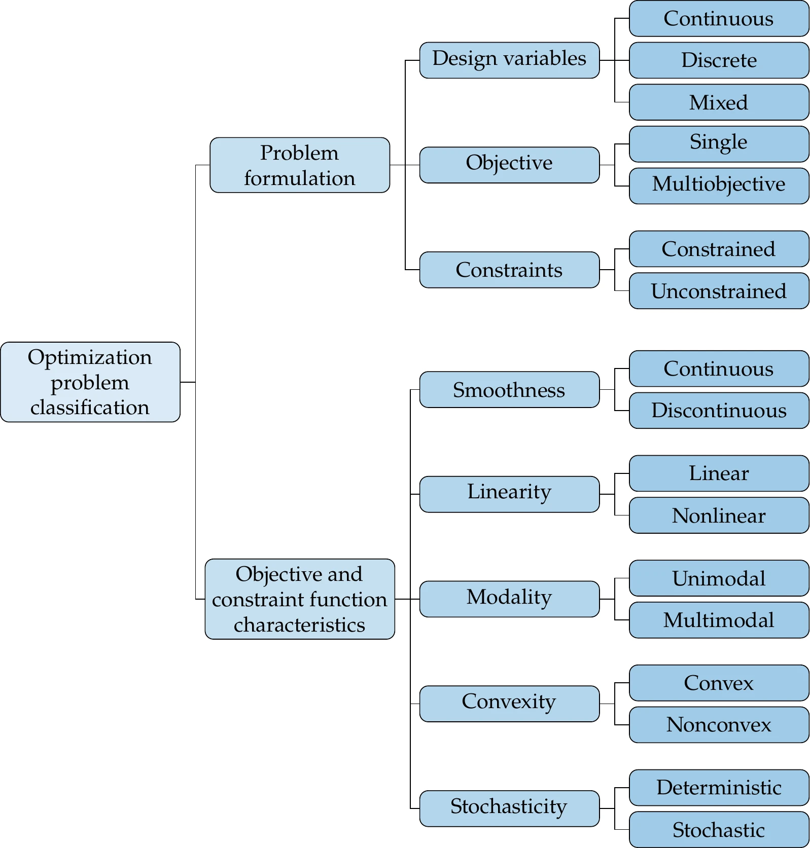
Figure 1.15:Optimization problems can be classified by attributes associated with the different aspects of the problem. The two main aspects are the problem formulation and the objective and constraint function characteristics.
In the problem formulation, the design variables can be either discrete or continuous. Most of this book assumes continuous design variables, but Chapter 8 provides an introduction to discrete optimization. When the design variables include both discrete and continuous variables, the problem is said to be mixed. Most of the book assumes a single objective function, but we explain how to solve multiobjective problems in Chapter 9. Finally, as previously mentioned, unconstrained problems are rare in engineering design optimization. However, we explain unconstrained optimization algorithms (Chapter 4) because they provide the foundation for constrained optimization algorithms (Chapter 5).
The characteristics of the objective and constraint functions also determine the type of optimization problem at hand and ultimately limit the type of optimization algorithm that is appropriate for solving the optimization problem.
In this section, we will view the function as a “black box”, that is, a computation for which we only see inputs (including the design variables) and outputs (including objective and constraints), as illustrated in Figure 1.16.
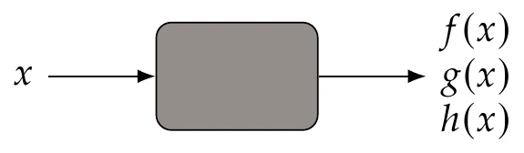
Figure 1.16:A model is considered a black box when we only see its inputs and outputs.
When dealing with black-box models, there is limited or no understanding of the modeling and numerical solution process used to obtain the function values. We discuss these types of models and how to solve them in Chapter 3, but here, we can still characterize the functions based purely on their outputs. The black-box view is common in real-world applications. This might be because the source code is not provided, the modeling methods are not described, or simply because the user does not bother to understand them.
In the remainder of this section, we discuss the attributes of objectives and constraints shown in Figure 1.15. Strictly speaking, many of these attributes cannot typically be identified from a black-box model. For example, although the model may appear smooth, we cannot know that it is smooth everywhere without a more detailed inspection. However, for this discussion, we assume that the black box’s outputs can be exhaustively explored so that these characteristics can be identified.
1.3.1 Smoothness
The degree of function smoothness with respect to variations in the design variables depends on the continuity of the function values and their derivatives. When the value of the function varies continuously, the function is said to be continuous. If the first derivatives also vary continuously, then the function is continuous, and so on. A function is smooth when the derivatives of all orders vary continuously everywhere in its domain. Function smoothness with respect to continuous design variables affects what type of optimization algorithm can be used. Figure 1.17 shows one-dimensional examples for a discontinuous function, a function, and a function.
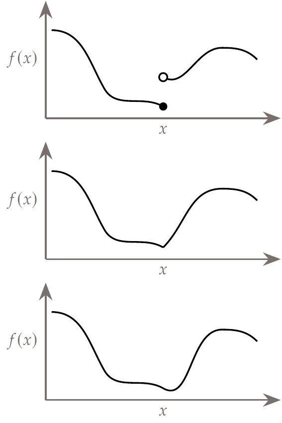
Figure 1.17:Discontinuous function (top), continuous function (middle), and continuous function (bottom).
As we will see later, discontinuities in the function value or derivatives limit the type of optimization algorithm that can be used because some algorithms assume , , and even continuity. In practice, these algorithms usually still work with functions that have only a few discontinuities that are located away from the optimum.
1.3.2 Linearity
The functions of interest could be linear or nonlinear. When both the objective and constraint functions are linear, the optimization problem is known as a linear optimization problem.
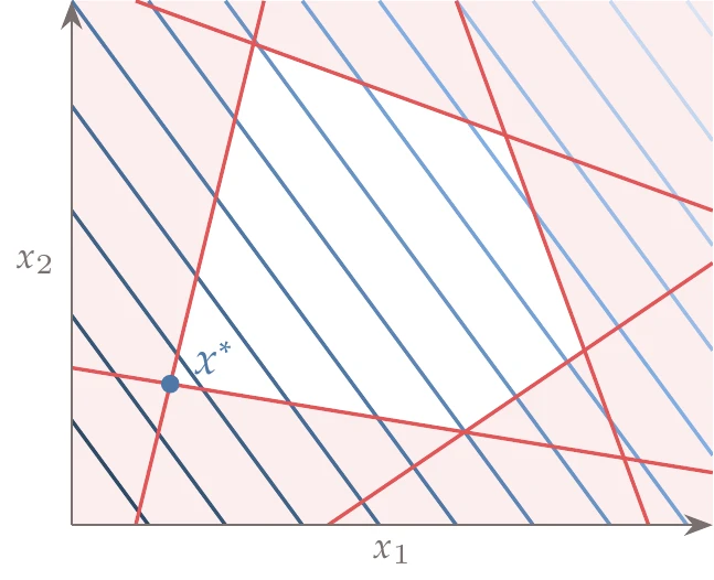
Figure 1.18:Example of a linear optimization problem in two dimensions.
These problems are easier to solve than general nonlinear ones, and there are entire books and courses dedicated to the subject. The first numerical optimization algorithms were developed to solve linear optimization problems, and there are many applications in operations research (see Chapter 2). An example of a linear optimization problem is shown in Figure 1.18.
When the objective function is quadratic and the constraints are linear, we have a quadratic optimization problem, which is another type of problem for which specialized solution methods exist.[9]Linear optimization and quadratic optimization are covered in Section 11.2, Section 11.3, and Section 5.5.
Although many problems can be formulated as linear or quadratic problems, most engineering design problems are nonlinear. However, it is common to have at least a subset of constraints that are linear, and some general nonlinear optimization algorithms take advantage of the techniques used to solve linear and quadratic problems.
1.3.3 Multimodality and Convexity
Functions can be either unimodal or multimodal. Unimodal functions have a single minimum, whereas multimodal functions have multiple minima. When we find a minimum without knowledge of whether the function is unimodal or not, we can only say that it is a local minimum; that is, this point is better than any point within a small neighborhood.
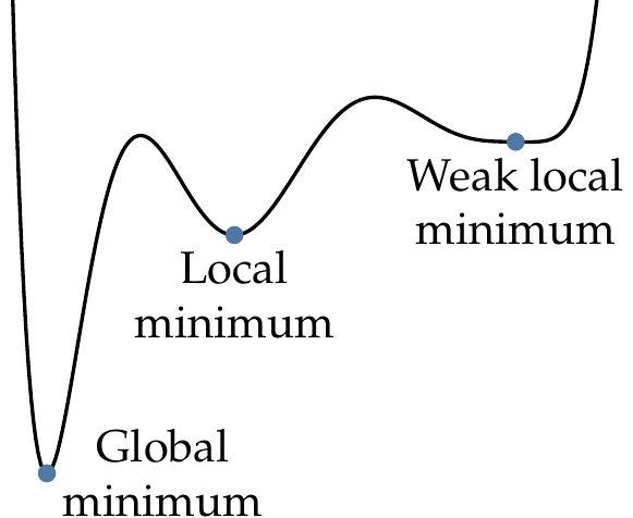
Figure 1.19:Types of minima.
When we know that a local minimum is the best in the whole domain (because we somehow know that the function is unimodal), then this is also the global minimum, as illustrated in Figure 1.19. Sometimes, the function might be flat around the minimum, in which case we have a weak minimum.
For functions involving more complicated numerical models, it is usually impossible to prove that the function is unimodal. Proving that such a function is unimodal would require evaluating the function at every point in the domain, which is computationally prohibitive. However, it much easier to prove multimodality—all we need to do is find two distinct local minima.
Just because a function is complicated or the design space has many dimensions, it does not mean that the function is multimodal. By default, we should not assume that a given function is either unimodal or multimodal. As we explore the problem and solve it starting from different points or using different optimizers, there are two main possibilities.
One possibility is that we find more than one minimum, thus proving that the function is multimodal. To prove this conclusively, we must make sure that the minima do indeed satisfy the mathematical optimality conditions with good enough precision.
The other possibility is that the optimization consistently converges to the same optimum. In this case, we can become increasingly confident that the function is unimodal with every new optimization that converges to the same optimum.[10]
Often, we need not be too concerned about the possibility of multiple local minima. From an engineering design point of view, achieving a local optimum that is better than the initial design is already a useful result.
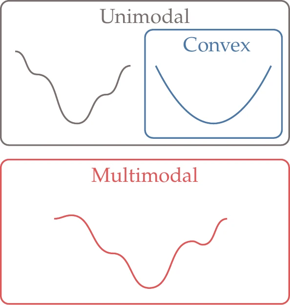
Figure 1.20:Multimodal functions have multiple minima, whereas unimodal functions have only one minimum. All multimodal functions are nonconvex, but not all unimodal functions are convex.
Convexity is a concept related to multimodality. A function is convex if all line segments connecting any two points in the function lie above the function and never intersect it. Convex functions are always unimodal. Also, all multimodal functions are nonconvex, but not all unimodal functions are convex (see Figure 1.20).
Convex optimization seeks to minimize convex functions over convex sets. Like linear optimization, convex optimization is another subfield of numerical optimization with many applications. When the objective and constraints are convex functions, we can use specialized formulations and algorithms that are much more efficient than general nonlinear algorithms to find the global optimum, as explained in Chapter 11.
1.3.4 Deterministic versus Stochastic
Some functions are inherently stochastic. A stochastic model yields different function values for repeated evaluations with the same input (Figure 1.21). For example, the numerical value from a roll of dice is a stochastic function.
Stochasticity can also arise from deterministic models when the inputs are subject to uncertainty. The input variables are then described as probability distributions, and their uncertainties need to be propagated through the model. For example, the bending stress in a beam may follow a deterministic model, but the beam’s geometric properties may be subject to uncertainty because of manufacturing deviations.
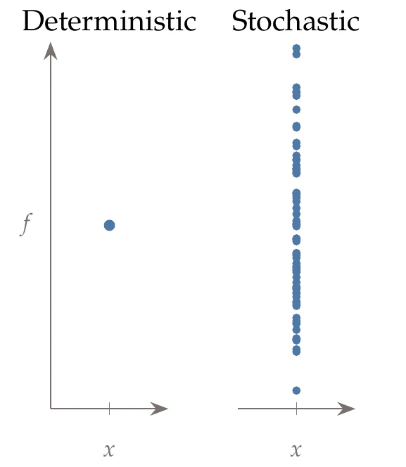
Figure 1.21:Deterministic functions yield the same output when evaluated repeatedly for the same input, whereas stochastic functions do not.
For most of this text, we assume that functions are deterministic, except in Chapter 12, where we explain how to perform optimization when the model inputs are uncertain.
1.4 Optimization Algorithms
No single optimization algorithm is effective or even appropriate for all possible optimization problems. This is why it is important to understand the problem before deciding which optimization algorithm to use. By “effective” algorithm, we mean that the algorithm can solve the problem, and secondly, it does so reliably and efficiently. Figure 1.22 lists the attributes for the classification of optimization algorithms, which we cover in more detail in the following discussion. These attributes are often amalgamated, but they are independent, and any combination is possible. In this text, we cover a wide variety of optimization algorithms corresponding to several of these combinations. However, this overview still does not cover a wide variety of specialized algorithms designed to solve specific problems where a particular structure can be exploited.
When multiple models are involved, we also need to consider how the models are coupled, solved, and integrated with the optimizer.
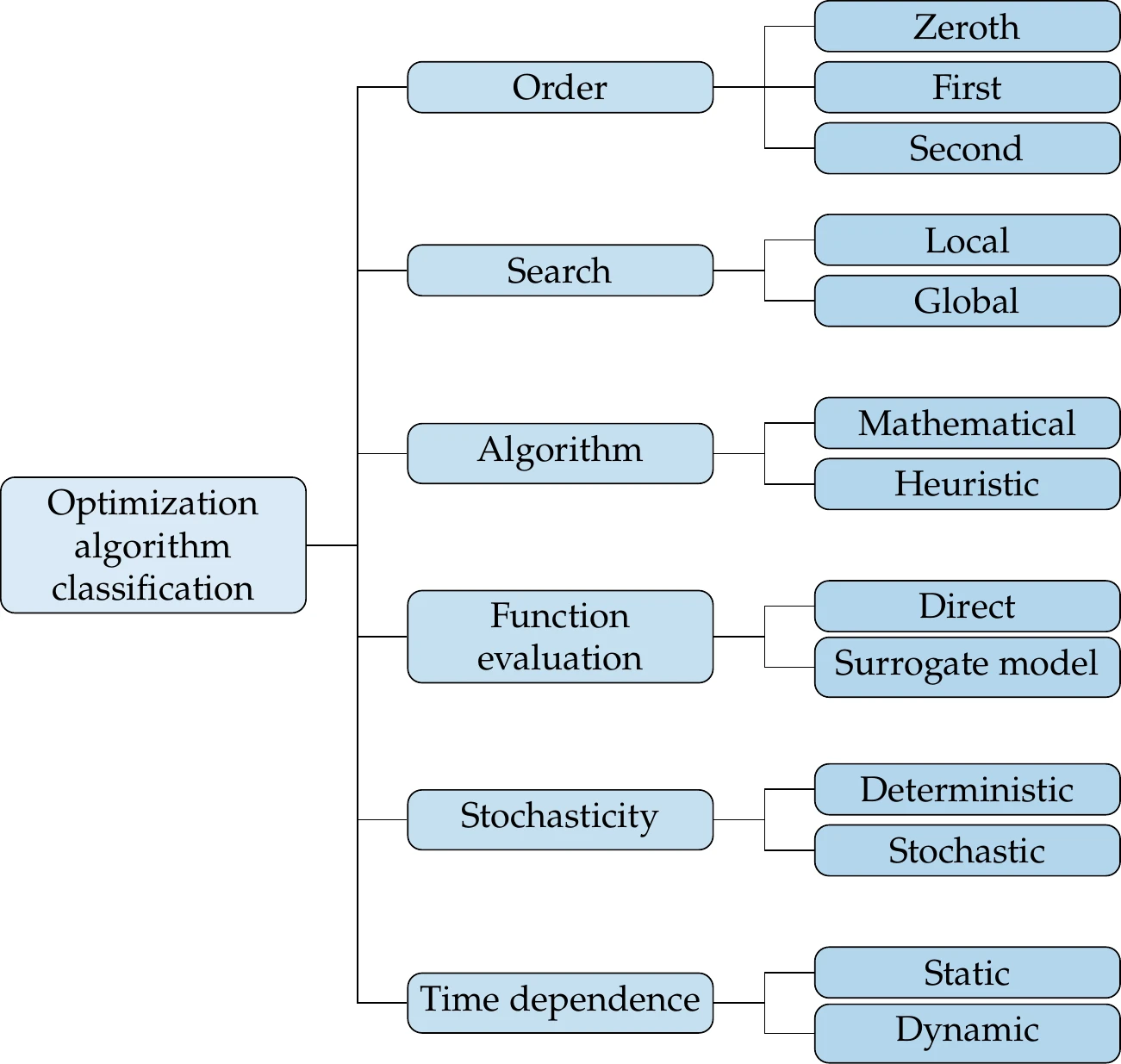
Figure 1.22:Optimization algorithms can be classified by using the attributes in the rightmost column. As in the problem classification step, these attributes are independent, and any combination is possible.
These considerations lead to different MDO architectures, which may involve multiple levels of optimization problems. Coupled models and MDO architectures are covered in Chapter 13.
1.4.1 Order of Information
At the minimum, an optimization algorithm requires users to provide the models that compute the objective and constraint values—zeroth-order information—for any given set of allowed design variables. We call algorithms that use only these function values gradient-free algorithms (also known as derivative-free or zeroth-order algorithms). We cover a selection of these algorithms in Chapter 7 and Chapter 8. The advantage of gradient-free algorithms is that the optimization is easier to set up because they do not need additional computations other than what the models for the objective and constraints already provide.
Gradient-based algorithms use gradients of both the objective and constraint functions with respect to the design variables—first-order information. The gradients provide much richer information about the function behavior, which the optimizer can use to converge to the optimum more efficiently.
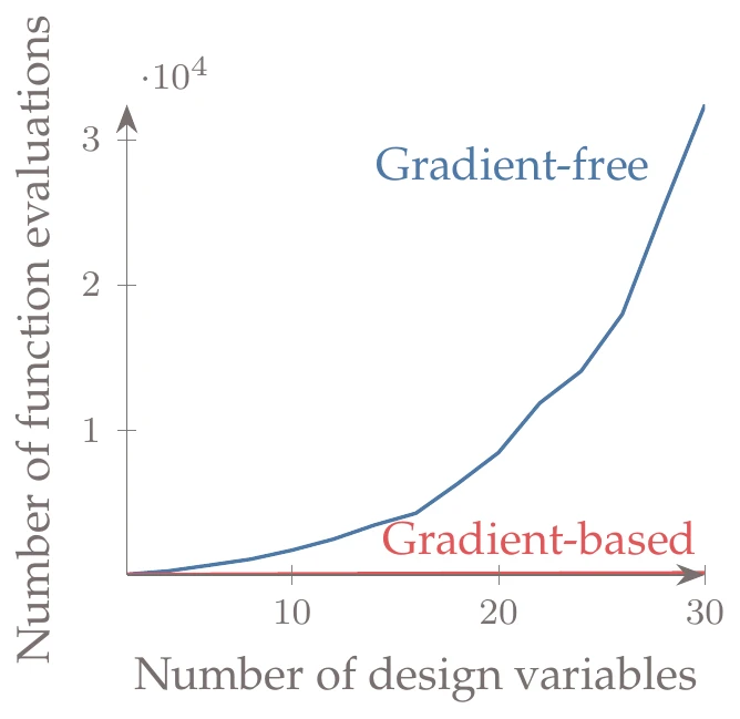
Figure 1.23:Gradient-based algorithms scale much better with the number of design variables. In this example, the gradient-based curve (with exact derivatives) grows from 67 to 206 function calls, but it is overwhelmed by the gradient-free curve, which grows from 103 function calls to over 32,000.
Figure 1.23 shows how the cost of gradient-based versus gradient-free optimization algorithms typically scales when the number of design variables increases. The number of function evaluations required by gradient-free methods increases dramatically, whereas the number of evaluations required by gradient-based methods does not increase as much and is many orders of magnitude lower for the larger numbers of design variables.
In addition, gradient-based methods use more rigorous criteria for optimality. The gradients are used to establish whether the optimizer converged to a point that satisfies mathematical optimality conditions, something that is difficult to verify in a rigorous way without gradients.
We first cover gradient-based algorithms for unconstrained problems in Chapter 4 and then extend them to constrained problems in Chapter 5. Gradient-based algorithms also include algorithms that use curvature—second-order information. Curvature is even richer information that tells us the rate of the change in the gradient, which provides an idea of where the function might flatten out.
There is a distinction between the order of information provided by the user and the order of information actually used in the algorithm. For example, a user might only provide function values to a gradient-based algorithm and rely on the algorithm to internally estimate gradients. Optimization algorithms estimate the gradients by requesting additional function evaluations for finite difference approximations (see Section 6.4). Gradient-based algorithms can also internally estimate curvature based on gradient values (see Section 4.4.4).
In theory, gradient-based algorithms require the functions to be sufficiently smooth (at least continuous). However, in practice, they can tolerate the occasional discontinuity, as long as this discontinuity is not near the optimum.
We devote a considerable portion of this book to gradient-based algorithms because they scale favorably with the number of design variables, and they have rigorous mathematical criteria for optimality. We also cover the various approaches for computing gradients in detail because the accurate and efficient computation of these gradients is crucial for the efficacy and efficiency of these methods (see Chapter 6).
Current state-of-the-art optimization algorithms also use second-order information to implement Newton-type methods for second-order convergence. However, these algorithms tend to build second-order information based on the provided gradients, as opposed to requiring users to provide the second-order information directly (see Section 4.4.4).
Because gradient-based methods require accurate gradients and smooth enough functions, they require more knowledge about the models and optimization algorithm than gradient-free methods. Chapters Chapter 3 through Chapter 6 are devoted to making the power of gradient-based methods more accessible by providing the necessary theoretical and practical knowledge.
1.4.2 Local versus Global Search
The many ways to search the design space can be classified as being local or global. A local search takes a series of steps starting from a single point to form a sequence of points that hopefully converges to a local optimum. In spite of the name, local methods can traverse large portions of the design space and can even step between convex regions (although this happens by chance). A global search tries to span the whole design space in the hope of finding the global optimum. As previously mentioned when discussing multimodality, even when using a global method, we cannot prove that any optimum found is a global one except for particular cases.
The classification of local versus global searches often gets conflated with the gradient-based versus gradient-free attributes because gradient-based methods usually perform a local search. However, these should be viewed as independent attributes because it is possible to use a global search strategy to provide starting points for a gradient-based algorithm. Similarly, some gradient-free algorithms are based on local search strategies.
The choice of search type is intrinsically linked to the modality of the design space. If the design space is unimodal, then a local search is sufficient because it converges to the global optimum. If the design space is multimodal, a local search converges to an optimum that might be local (or global if we are lucky enough). A global search increases the likelihood that we converge to a global optimum, but this is by no means guaranteed.
1.4.3 Mathematical versus Heuristic
There is a big divide regarding the extent to which an algorithm is based on provable mathematical principles versus heuristics. Optimization algorithms require an iterative process, which determines the sequence of points evaluated when searching for an optimum, and optimality criteria, which determine when the iterative process ends. Heuristics are rules of thumb or commonsense arguments that are not based on a strict mathematical rationale.
Gradient-based algorithms are usually based on mathematical principles, both for the iterative process and for the optimality criteria. Gradient-free algorithms are more evenly split between the mathematical and heuristic for both the optimality criteria and the iterative procedure. The mathematical gradient-free algorithms are often called derivative-free optimization algorithms. Heuristic gradient-free algorithms include a wide variety of nature-inspired algorithms (see Section 7.2).
Heuristic optimality criteria are an issue because, strictly speaking, they do not prove that a given point is a local (let alone global) optimum; they are only expected to find a point that is “close enough”. This contrasts with mathematical optimality criteria, which are unambiguous about (local) optimality and converge to the optimum within the limits of the working precision.
This is not to suggest that heuristic methods are not useful. Finding a better solution is often desirable regardless of whether or not it is strictly optimal. Not converging tightly to optimality criteria does, however, make it harder to compare results from different methods.
Iterative processes based on mathematical principles tend to be more efficient than those based on heuristics. However, some heuristic methods are more robust because they tend to make fewer assumptions about the modality and smoothness of the functions and handle noisy functions more effectively.
Most algorithms mix mathematical arguments and heuristics to some degree. Mathematical algorithms often include constants whose values end up being tuned based on experience. Conversely, algorithms primarily based on heuristics sometimes include steps with mathematical justification.
1.4.4 Function Evaluation
The optimization problem setup that we described previously assumes that the function evaluations are obtained by solving numerical models of the system. We call these direct function evaluations. However, it is possible to create surrogate models (also known as metamodels) of these models and use them in the optimization process. These surrogates can be interpolation-based or projection-based models. Surrogate-based optimization is discussed in Chapter 10.
1.4.5 Stochasticity
This attribute is independent of the stochasticity of the model that we mentioned previously, and it is strictly related to whether the optimization algorithm itself contains steps that are determined at random or not.
A deterministic optimization algorithm always evaluates the same points and converges to the same result, given the same initial conditions. In contrast, a stochastic optimization algorithm evaluates a different set of points if run multiple times from the same initial conditions, even if the models for the objective and constraints are deterministic. For example, most evolutionary algorithms include steps determined by generating random numbers. Gradient-based algorithms are usually deterministic, but some exceptions exist, such as stochastic gradient descent (see Section 10.5).
1.4.6 Time Dependence
In this book, we assume that the optimization problem is static. This means that we formulate the problem as a single optimization and solve the complete numerical model at each optimization iteration. In contrast, dynamic optimization problems solve a sequence of optimization problems to make decisions at different time instances based on information that becomes available as time progresses.
For some problems that involve time dependence, we can perform time integration to solve for the entire time history of the states and then compute the objective and constraint function values for an optimization iteration. This means that every optimization iteration requires solving for the entire time history. An example of this type of problem is a trajectory optimization problem where the design variables are the coordinates representing the path, and the objective is to minimize the total energy expended to get to a given destination.4 Although such a problem involves a time dependence, we still classify it as static because we solve a single optimization problem. As a more specific example, consider a car going around a racetrack. We could optimize the time history of the throttle, braking, and steering of a car to get a trajectory that minimizes the total time in a known racetrack for fixed conditions. This is an open-loop optimal control problem because the car control is predetermined and does not react to any disturbances.
For dynamic optimization problems (also known as dynamic programming), the design variables are decisions made in a sequence of time steps.56 The decision at a given time step is influenced by the decisions and system states from previous steps. Sometimes, the decision at a given time step also depends on a prediction of the states a few steps into the future.
The car example that we previously mentioned could also be a dynamic optimization problem if we optimized the throttle, braking, or steering of a car at each time instance in response to some measured output. We could, for example, maximize the instantaneous acceleration based on real-time acceleration sensor information and thus react to varying conditions, such as surface traction. This is an example of a closed-loop (or feedback) optimal control problem, a type of dynamic optimization problem where a control law is optimized for a dynamical system over a period of time.
Dynamic optimization is not covered in this book, except in the context of discrete optimization (see Section 8.5). Different approaches are used in general, but many of the concepts covered here are instrumental in the numerical solution of dynamic optimization and optimal control problems.
1.5 Selecting an Optimization Approach
This section provides guidance on how to select an appropriate approach for solving a given optimization problem. This process cannot always be distilled to a simple decision tree; however, it is still helpful to have a framework as a first guide. Many of these decisions will become more apparent as you progress through the book and gain experience, so you may want to revisit this section periodically. Eventually, selecting an appropriate methodology will become second nature.
Figure 1.24 outlines one approach to algorithm selection and also serves as an overview of the chapters in this book. The first two characteristics in the decision tree (convex problem and discrete variables) are not the most common within the broad spectrum of engineering optimization problems, but we list them first because they are the more restrictive in terms of usable optimization algorithms.
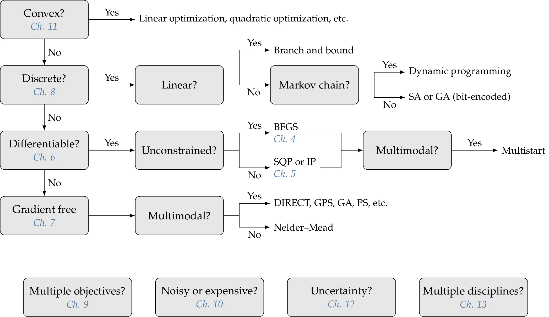
Figure 1.24:Decision tree for selecting an optimization algorithm.
The first node asks about convexity. Although it is often not immediately apparent if the problem is convex, with some experience, we can usually discern whether we should attempt to reformulate it as a convex problem. In most instances, convexity occurs for problems with simple objectives and constraints (e.g., linear or quadratic), such as in control applications where the optimization is performed repeatedly. A convex problem can be solved with general gradient-based or gradient-free algorithms, but it would be inefficient not to take advantage of the convex formulation structure if we can do so.
The next node asks about discrete variables. Problems with discrete design variables are generally much harder to solve, so we might consider alternatives that avoid using discrete variables when possible. For example, a wind turbine’s position in a field could be posed as a discrete variable within a discrete set of options. Alternatively, we could represent the wind turbine’s position as a continuous variable with two continuous coordinate variables. That level of flexibility may or may not be desirable but generally leads to better solutions. Many problems are fundamentally discrete, and there is a wide variety of available methods.
Next, we consider whether the model is continuous and differentiable or can be made smooth through model improvements. If the problem is high dimensional (more than a few tens of variables as a rule of thumb), gradient-free algorithms are generally intractable and gradient-based algorithms are preferable. We would either need to make the model smooth enough to use a gradient-based algorithm or reduce the problem dimensionality to use a gradient-free algorithm. Another alternative if the problem is not readily differentiable is to use surrogate-based optimization (the box labeled “Noisy or expensive” in Figure 1.24). If we go the surrogate-based optimization route, we could still use a gradient-based approach to optimize the surrogate model because most such models are differentiable. Finally, for problems with a relatively small number of design variables, gradient-free methods can be a good fit. Gradient-free methods have the largest variety of algorithms, and a combination of experience and testing is needed to determine an appropriate algorithm for the problem at hand.
The bottom row in Figure 1.24 lists additional considerations: multiple objectives, surrogate-based optimization for noisy (nondifferentiable) or computationally expensive functions, optimization under uncertainty in the design variables and other model parameters, and MDO.
1.6 Notation
We do not use bold font to represent vectors or matrices. Instead, we follow the convention of many optimization and numerical linear algebra books, which try to use Greek letters (e.g., and ) for scalars, lowercase roman letters (e.g., and ) for vectors, and capitalized roman letters (e.g., and ) for matrices.
There are exceptions to this notation because of the wide variety of topics covered in this book and a desire not to deviate from the standard conventions used in each field. We explicitly note these exceptions as needed. For example, the objective function is a scalar function and the Lagrange multipliers ( and ) are vectors.
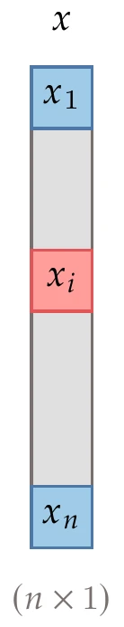
Figure 1.25:An -vector, .
By default, a vector is a column vector, and thus is a row vector. We denote the th element of the vector as , as shown in Figure 1.25. For more compact notation, we may write a column vector horizontally, with its components separated by commas, for example, . We refer to a vector with components as an -vector, which is equivalent to writing .
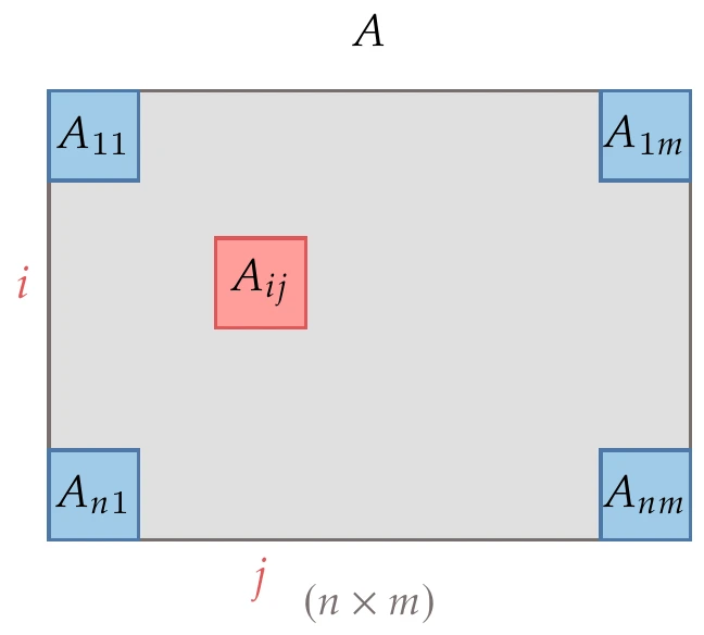
Figure 1.26:An matrix, .
An matrix has rows and columns, which is equivalent to defining . The matrix element is the element in the th row of the the column, as shown in Figure 1.26. Occasionally, additional letters beyond and are needed for indices, but those are explicitly noted when used.
The subscript usually refers to iteration number. Thus, is the complete vector at iteration . The subscript zero is used for the same purpose, so would be the complete vector at the initial iteration. Other subscripts besides those listed are used for naming.
A superscript star () refers to a quantity at the optimum.
1.7 Summary
Optimization is compelling, and there are opportunities to apply it everywhere. Numerical optimization fully automates the design process but requires expertise in the problem formulation, optimization algorithm selection, and the use of that algorithm. Finally, design expertise is also required to interpret and critically evaluate the results given by the optimization.
There is no single optimization algorithm that is effective in the solution of all types of problems. It is crucial to classify the optimization problem and understand the optimization algorithms’ characteristics to select the appropriate algorithm to solve the problem.
In seeking a more automated design process, we must not dismiss the value of engineering intuition, which is often difficult (if not impossible) to convert into a rigid problem formulation and algorithm.
Problems
The evaluation of a given design in engineering is often called the analysis. Engineers and computer scientists also refer to it as simulation.
Some texts call these decision variables or simply variables.
This is not to be confused with the continuity of the objective and constraint functions, which we discuss in Section 1.3.
Inverting the function () is another way to turn a maximization problem into a minimization problem, but it is generally less desirable because it alters the scale of the problem and could introduce a divide-by-zero problem.
The simple models used in this example are described in Section D.1.6.
A strict inequality, , is never used because then could be arbitrarily close to the equality. Because the optimum is at for an active constraint, the exact solution would then be ill-defined from a mathematical perspective. Also, the difference is not meaningful when using finite-precision arithmetic (which is always the case when using a computer).
Instead of “by varying”, some textbooks use “with respect to” or “w.r.t.” as shorthand.
Optimization software resources include the optimization toolboxes in MATLAB,
scipy.optimize.minimizein Python,Optim.jlorIpopt.jlin Julia,NLoptfor multiple languages, and the Solver add-in in Microsoft Excel. The pyOptSparse framework provides a common Python wrapper for many existing optimization codes and facilitates the testing of different methods.1SNOW.jlwraps a few optimizers and multiple derivative computation methods in Julia.Historically, optimization problems were referred to as programming problems, so much of the existing literature refers to linear optimization as linear programming and similarly for other types of optimization.
- Wu, N., Kenway, G., Mader, C. A., Jasa, J., & Martins, J. R. R. A. (2020). pyOptSparse: A Python framework for large-scale constrained nonlinear optimization of sparse systems. Journal of Open Source Software, 5(54), 2564. 10.21105/joss.02564
- Lyu, Z., Kenway, G. K. W., & Martins, J. R. R. A. (2015). Aerodynamic Shape Optimization Investigations of the Common Research Model Wing Benchmark. AIAA Journal, 53(4), 968–985. 10.2514/1.J053318
- He, X., Li, J., Mader, C. A., Yildirim, A., & Martins, J. R. R. A. (2019). Robust aerodynamic shape optimization—From a circle to an airfoil. Aerospace Science and Technology, 87, 48–61. 10.1016/j.ast.2019.01.051
- Betts, J. T. (1998). Survey of numerical methods for trajectory optimization. Journal of Guidance, Control, and Dynamics, 21(2), 193–207. 10.2514/2.4231
- Bryson, A. E., & Ho, Y. C. (1969). Applied Optimal Control; Optimization, Estimation, and Control. Blaisdell Publishing. https://books.google.com/books/about/Applied_Optimal_Control.html
- Bertsekas, D. P. (1995). Dynamic Programming and Optimal Control. Athena Scientific. https://books.google.com/books/about/Dynamic_Programming_and_Optimal_Control.html