10 Surrogate-Based Optimization
A surrogate model, also known as a response surface model or metamodel, is an approximate model of a functional output that represents a “curve fit” to some underlying data. The goal of a surrogate model is to build a model that is much faster to compute than the original function, but that still retains sufficient accuracy away from known data points.
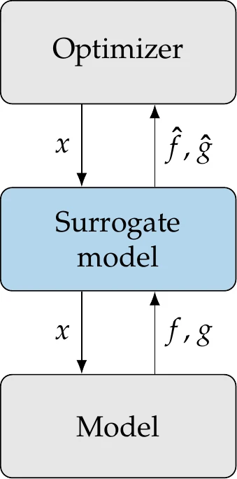
Figure 10.1:Surrogate-based optimization replaces the original model with a surrogate model in the optimization process.
Surrogate-based optimization (SBO) performs optimization using the surrogate model, as shown in Figure 10.1. When used in optimization, the surrogate might define the full optimization model (i.e., the inputs are design variables, and the outputs are objective and constraint functions), or the surrogate could be just a component of the overall model. SBO is more targeted than the broader field of surrogate modeling. Instead of aiming for a globally accurate surrogate, SBO just needs the surrogate model to be accurate enough to lead the optimizer to the true optimum.
In SBO, the surrogate model is usually improved during optimization as needed but can sometimes be constructed beforehand and remain fixed during optimization. Some optimization algorithms interrogate both the surrogate model and the original model, an approach that is sometimes called surrogate-assisted optimization.
10.1 When to Use a Surrogate Model
There are various scenarios for which surrogate models are helpful. One scenario is when the original model is computationally expensive. Surrogate models can be queried with minimal computational cost, but constructing them requires multiple evaluations of the original model. Suppose the number of evaluations needed to build a sufficiently accurate surrogate model is less than that needed to optimize the original model directly. In that case, SBO may be a worthwhile option. Constructing a surrogate model becomes even more compelling when it is reused in multiple optimizations.
Surrogate modeling can be effective in handling noisy models because they create a smooth representation of noisy data. This can be particularly advantageous when using gradient-based optimization.
One scenario that leads to both expensive evaluation and noisy output is experimental data. When the model data are experimental and the optimizer cannot query the experiment in an automated way, we can construct a surrogate model based on the experimental data. Then, the optimizer can query the surrogate model in the optimization.
Surrogate models are also helpful when we want to understand the design space, that is, how the objective and constraints (outputs) vary with respect to the design variables (inputs). By constructing a continuous model over discrete data, we obtain functional relationships that can be visualized more effectively.
When multiple sources of data are available, surrogate models can fuse the data to build a single model. The data could come from numerical models with different levels of fidelity or experimental data. For example, surrogate models can calibrate numerical model data using experimental data. This is helpful because experimental data is usually much more scarce than numerical data. The same reasoning applies to low- versus high-fidelity numerical data.
One potential issue with surrogate models is the curse of dimensionality, which refers to poor scalability with the number of inputs. The larger the number of inputs, the more model evaluations are needed to construct a surrogate model that is accurate enough. Therefore, the reasons for using surrogate models cited earlier might not be enough if the optimization problem has a large number of design variables.
The SBO process is shown in Figure 10.2. First, we use sampling methods to choose the initial points to evaluate the function or conduct experiments. These points are sometimes referred to as training data. Next, we build a surrogate model from the sampled points. We can then perform optimization by querying the surrogate model. Based on the results of the optimization, we include additional points in the sample and reconstruct the surrogate (infill).
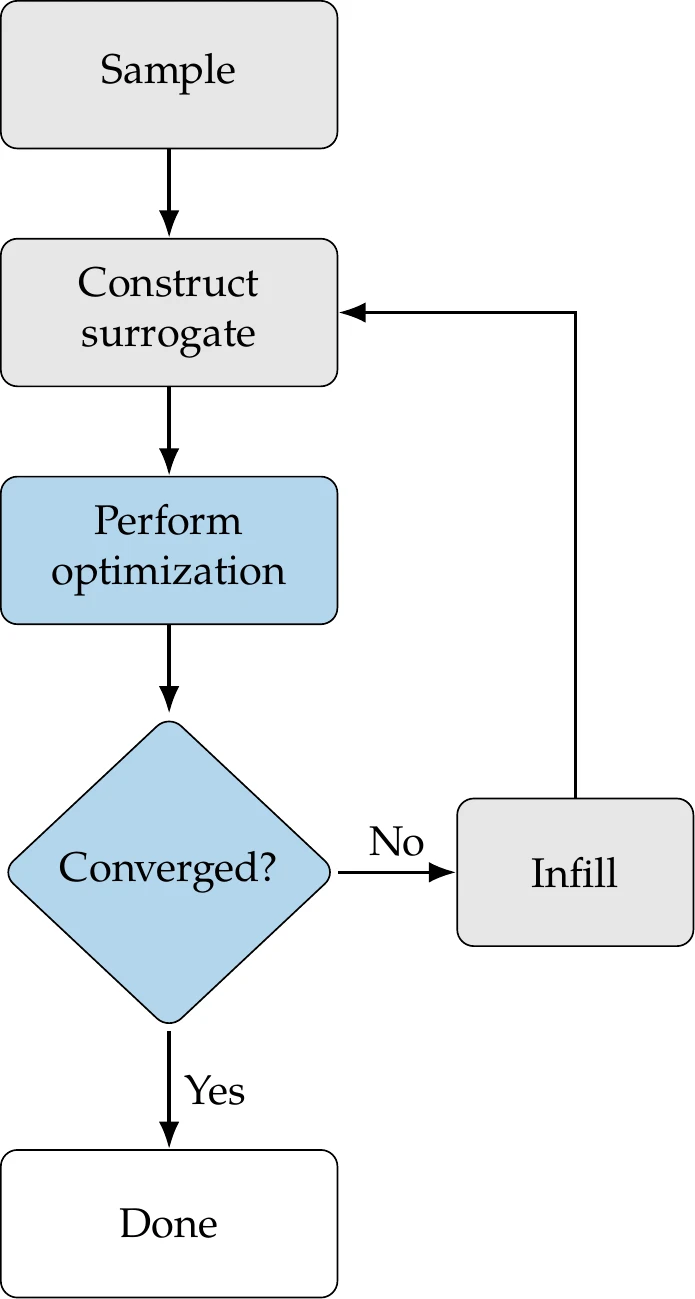
Figure 10.2:Overview of surrogate-based optimization procedure.
We repeat this process until some convergence criterion or a maximum number of iterations is reached. In some procedures, infill is omitted; the surrogate is entirely constructed upfront and not subsequently updated.
The optimization step can be performed using any of the methods we covered previously. Because surrogate models are smooth and their gradients are easily computed, gradient-based optimization is preferred (see Chapter 4). However, some surrogate models can be highly multimodal, in which case a global search is preferred, either using gradient-based with multistart (see Tip 4.8) or a global gradient-free method (see Chapter 7).
This chapter discusses sampling, constructing a surrogate, and infill with some associated optimization strategies. We devote separate sections to two surrogate modeling methods that are more involved and widely used: kriging and deep neural nets. Many of the concepts discussed in this chapter have a wide range of applications beyond optimization.
10.2 Sampling
Sampling methods, also known as sampling plans, select the evaluation points to construct the initial surrogate. These evaluation points must be chosen carefully. A straightforward approach is full factorial sampling, where we discretize each dimension and evaluate at all combinations of the resulting grid. This is not efficient because it scales exponentially with the number of input variables.
Example 10.1 highlights one of the significant challenges of sampling methods: the curse of dimensionality.
For SBO, even with better sampling plans, using a large number of variables is costly. We need to identify the most important or most influential variables. Knowledge of the particular domain is helpful, as is exploring the magnitude of the entries in a gradient vector (Chapter 6) across multiple points in the domain. We can use various strategies to help us decide which variables matter most, but for our purposes, we assume that the most influential variables have already been determined so that the dimensionality is reasonable. Having selected a set of variables, we are now interested in sampling methods that characterize the design space of interest more efficiently than full factorial sampling.
In addition to their use in SBO, the sampling strategies discussed in this section are useful in many other applications, including various applications discussed in this book: initializing a genetic algorithm (Section 7.6), particle swarm optimization (Section 7.7) or a multistart gradient-based algorithm (Tip 4.8), or choosing the points to run in a Monte Carlo simulation (Section 12.3.3). Because the function behavior at each sample is independent, we can efficiently parallelize the evaluation of the functions.
10.2.1 Latin Hypercube Sampling
Latin hypercube sampling (LHS) is a popular sampling method that is built on a random process but is more effective and efficient than pure random sampling. Random sampling scales better than full factorial searches, but it tends to exhibit clustering and requires many points to reach the desired distribution (i.e., the law of large numbers). For example, Figure 10.3 compares 50 randomly generated points across uniform distributions in two dimensions versus Latin hypercube sampling. In random sampling, each sample is independent of past samples, but in LHS, we choose all samples beforehand to ensure a well-spread distribution.
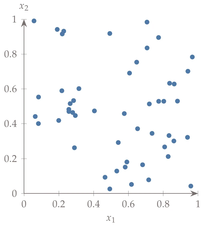
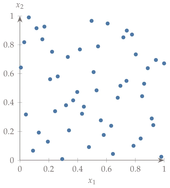
Figure 10.3a:Contrast between random and Latin hypercube sampling with 50 points using uniform distributions.
To describe the methodology, consider two random variables with bounds, whose design space we can represent as a square.

Figure 10.4:A two-dimensional design space divided into eight intervals in each dimension.
Say we wanted only eight samples; we could divide the design space into eight intervals in each dimension, generating the grid of cells shown in Figure 10.4.
A full factorial search would identify a point in each cell, but that does not scale well. To be as efficient as possible and still cover the variation, we would want each row and each column to have one sample in it. In other words, the projection of points onto each dimension should be uniform. For example, the left side of Figure 10.5 shows the projection of a uniform LHS onto each dimension. We see that the points create a uniformly spread histogram.
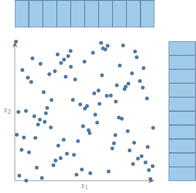
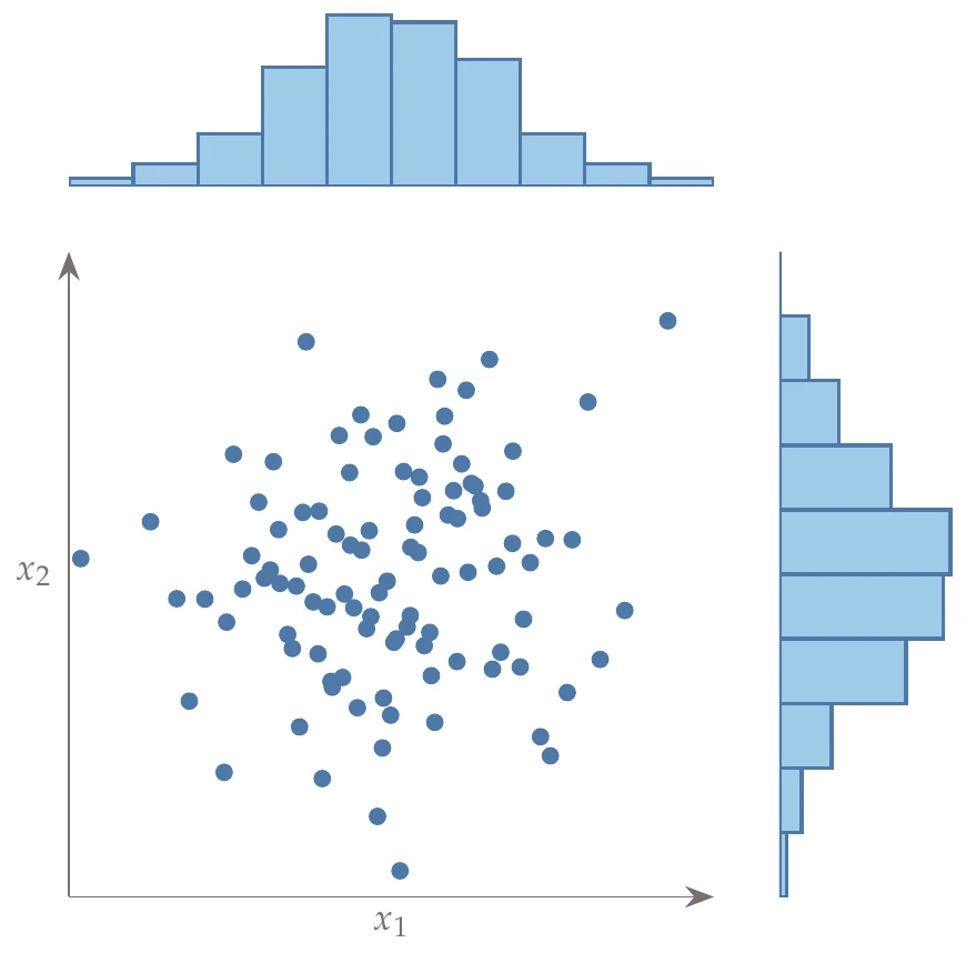
Figure 10.5a:Example LHS with projections onto the axes.
The concept where one and only one point exists in any given row or column is called a Latin square, and the generalization to higher dimensions is called a Latin hypercube. There are many ways to achieve this, and some choices are better than others. Consider the sampling plan shown on the left of Figure 10.6. This plan meets our criteria but clearly does not fill the space and likely will not capture the relationships between design parameters well. Alternatively, the right side of Figure 10.6 has a sample in each row and column while also spanning the space much more effectively.
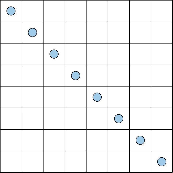
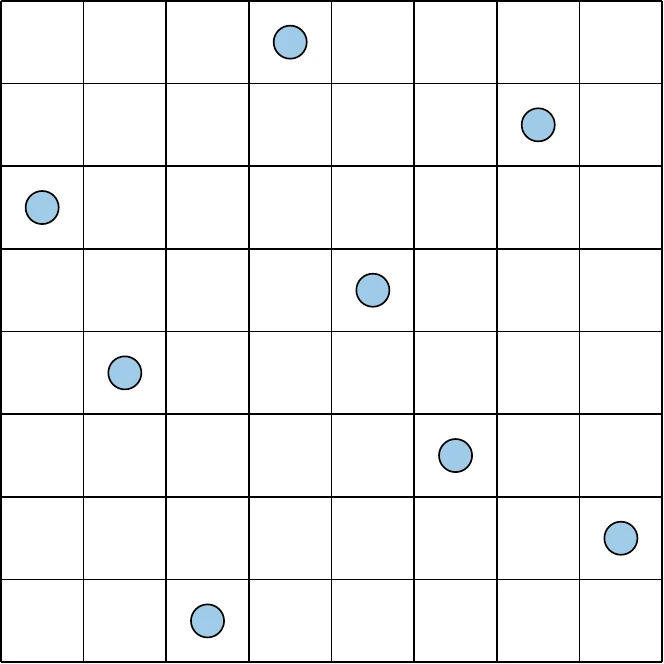
Figure 10.6a:Contrasting sampling strategies that both fulfill the uniform projection requirement.
LHS can be posed as an optimization problem where we seek to maximize the distance between the samples.
The constraint is that the projection on each axis must follow a chosen probability distribution. The specified distribution is often uniform, as in the previous examples, but it could also be any distribution, such as a normal distribution, as shown on the right side of Figure 10.5. This optimization problem does not have a unique solution, so random processes are used to determine the combination of points. Additionally, points are not usually placed in cell centers but at a random location within a given cell to allow for the possibility of reaching any point in the domain. The advantage of the LHS approach is that rather than relying on the law of large numbers to fill out our chosen probability distributions, we enforce it as a constraint. This method may still require many samples to characterize the design space accurately, but it usually requires far fewer than pure random sampling.
Instead of defining LHS as an optimization problem, a much simpler approach is typically used in which we ensure one sample per interval, but we rely on randomness to choose point combinations. Although this does not necessarily yield a maximum spread, it works well in practice and is simple to implement. Before discussing the algorithm, we discuss how to generate other distributions besides just uniform distributions.
We can convert from uniformly sampled points to an arbitrary distribution using a technique called inversion sampling.
Assume that we want to generate samples from an arbitrary probability density function (PDF) or, equivalently, from the corresponding cumulative distribution function (CDF) .[1]The probability integral transform states that for any continuous CDF, , the variable is uniformly distributed (a simple proof, but it is not shown here to avoid introducing additional notation). The procedure is to randomly sample from a uniform distribution (e.g., generate ), then compute the corresponding such that , which we denote as . This latter step is known as an inverse CDF, a percent-point function, or a quantile function. This process is depicted in Figure 10.7 for a normal distribution. This same procedure allows us to use LHS with any distribution, simply by generating the samples on a uniform distribution.
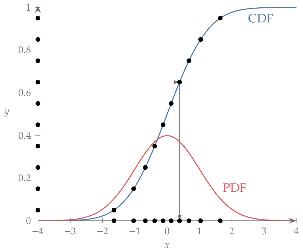
Figure 10.7:An example of inversion sampling with a normal distribution. A few uniform samples are shown on the -axis. The points are evaluated by the inverse CDF, represented by the arrows passing through the CDF for a normal distribution. If enough samples are drawn, the resulting distribution will be the PDF of a normal distribution.
A typical algorithm is described in Algorithm 10.1. For each axis, we partition the CDF in evenly spaced regions (evenly spaced along the CDF, which means that each region is equiprobable). We generate a random number within each evenly spaced interval, where 0 corresponds to the bottom of the interval and 1 to the top. We then evaluate the inverse CDF as described previously so that the points match our specified distribution (the CDF for a uniform distribution is just a line , so the output is not changed). Next, the column of points for that axis is randomly permuted. This process is repeated for each axis according to its specified probability distribution.
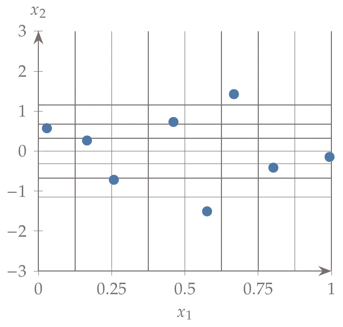
Figure 10.8:An example from the LHS algorithm showing uniform distribution in and a Gaussian distribution in with eight sample points. The equiprobable bins are shown as grid lines.
An example using Algorithm 10.1 for eight points is shown in Figure 10.8. In this example, we use a uniform distribution for and a normal distribution for . There is one point in each equiprobable interval. As stated before, randomness does not necessarily ensure a good spread, but optimizing the spread is difficult because the function is highly multimodal. Instead, to encourage high spread, we could generate multiple Latin hypercube samples with this algorithm and select the one with the largest sum of the distance between points.
10.2.2 Low-Discrepancy Sequences
Low-discrepancy sequences generate deterministic sequences of points that are well spread. Each new point added in the sequence maintains low discrepancy—discrepancy refers to the variation in point density throughout the domain. Hence, a low-discrepancy set is close to even density (i.e., well spread). These sequences are called quasi-random because they often serve as suitable replacements for applications that use random sequences, but they are not random or even pseudo-random.
An advantage of low-discrepancy sequences over LHS is that most of the approaches do not require selecting all the samples beforehand. These methods generate deterministic sequences; in other words, we generate the same sequence of points whether we choose them beforehand or add more later. This property is particularly advantageous in iterative procedures. We may choose an initial sampling plan and add more well-spread points to the sample later. This is not necessarily an advantage for the methods of this chapter because the optimization drives the selection of new points rather than continuing to seek spread-out samples. However, this feature is useful for other applications, such as quadrature, Monte Carlo simulations, and other problems where an iterative sampling process is used to determine statistical convergence (see Section 12.3). Low-discrepancy sequences add more points that are well spread without having to throw out the existing samples. Even in non-iterative procedures, these sampling strategies can be a useful alternative.
Several of these sequences are built on generalizations of the one-dimensional van der Corput sequence to more than one dimension. Such sequences are defined by representing an integer in a given integer base (the van der Corput sequence is always base 2):
If the base is 2, this is just a standard binary sequence (Section 7.6.1). After determining the relevant coefficients (), the element of the sequence is
An algorithm to generate an element in this sequence, also known as a radical inverse function for base , is given in Algorithm 10.2.
For base 2, the sequence is as follows:
The interval is divided in half, and then each subinterval is also halved, with new points spreading out across the domain (see Figure 10.9).
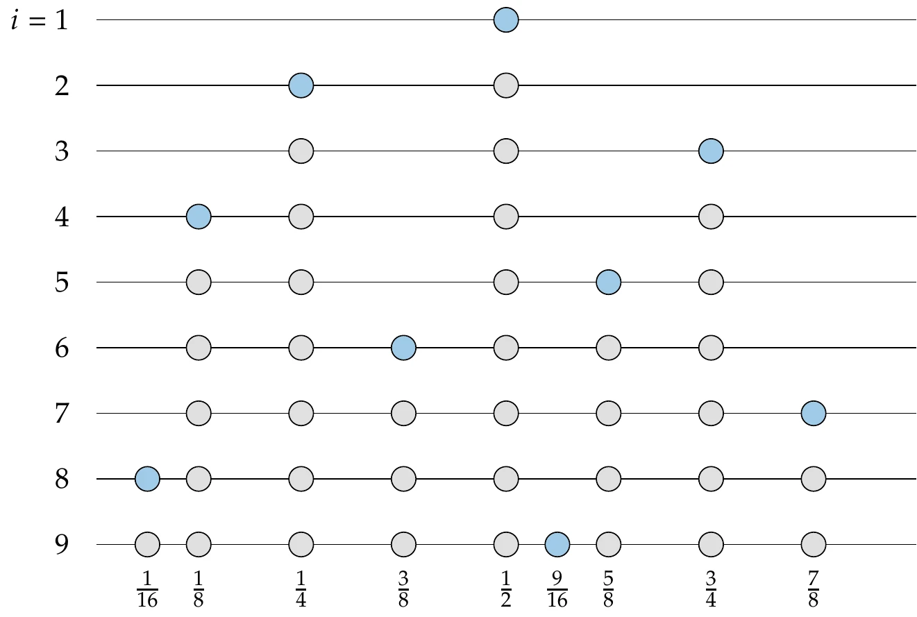
Figure 10.9:Van Der Corput sequence.
Similarly, for base 3, the interval is split into thirds, then each subinterval is split into thirds, and so on:
Halton Sequence
A Halton sequence uses pairwise prime numbers (larger than 1) for the base of each dimension of the problem.[2]The point in the Halton sequence is
where the set is pairwise prime. As an example in two dimensions, Figure 10.10 shows 30 generated points of the Halton sequence where uses base 2, and uses base 3, and then a subsequent 20 generated points are added (in another color), showing the reuse of existing points.
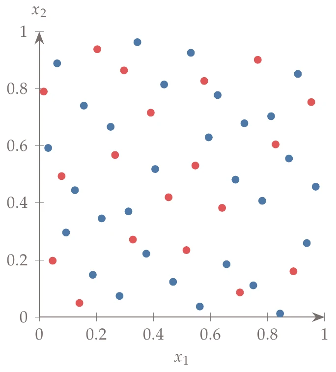
Figure 10.10:Halton sequence with base 2 for and base 3 for . First, 30 points are selected (in blue), and then 20 points are added (in red). These points would be identical to 50 points chosen at once.
If the dimensionality of the problem is high, then some of the base combinations lead to points that are highly correlated and thus undesirable for a sampling plan. For example, the left of Halton sequence with base 17 for and base 19 for . shows 50 generated points where uses base 17, and uses base 19. To avoid this issue, we can use a scrambled Halton sequence.
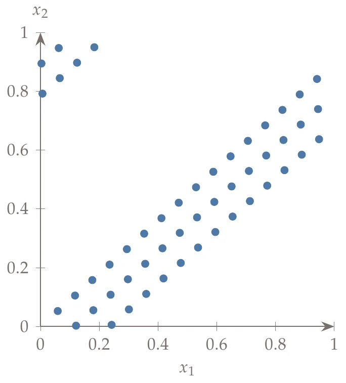
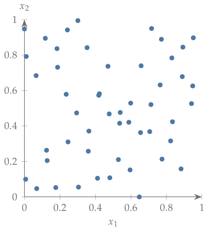
Figure 10.11a:Halton sequence with base 17 for and base 19 for .
Scrambling can be accomplished by generating a permutation array containing a random permutation of the integers . Then, rather than using the integers directly in Equation 10.2, we use the entries of as the indices of the permutation array. If is the permutation array, we have:
The permutation array is fixed for all digits and for all points in the domain. The right side of Halton sequence with base 17 for and base 19 for . shows the same example (with base 17 and base 19) but with scrambling to weaken the strong correlations.
Hammersley Sequence
The Hammersley sequence is closely related to the Halton sequence. However, it provides better spacing if we know beforehand the number of points () that we are going to use. This approach only needs bases (still pairwise prime) because the first dimension uses regular spacing:
Because this sequence needs to know the number of points () beforehand, it is less useful for iterative procedures.
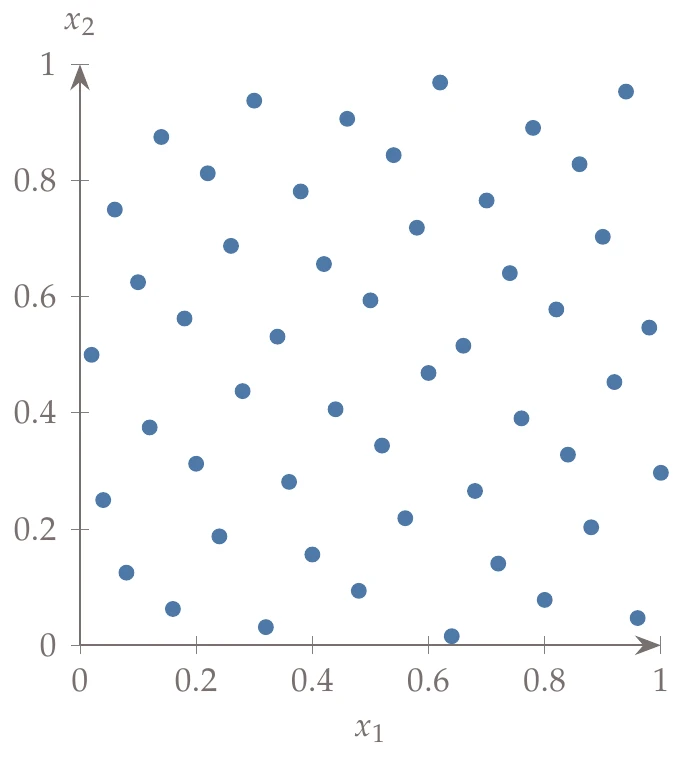
Figure 10.12:Hammersley sequence with base 2 for the -axis.
However, the implementation is straightforward, and so it may still be a useful alternative to LHS. Figure 10.12 shows 50 points generated from a Hammersley sequence where the -axis uses base 2.
Other Sequences
A wide variety of other low-discrepancy sequences exist. The Faure sequence is similar to the Halton, but it uses the same base for all dimensions and uses permutation scrambling for each dimension instead.12 Sobol sequences use base 2 sequences but with a reordering based on “direction numbers”.3 Niederreiter sequences are effectively a generalization of Sobol sequences to other bases.4
10.3 Constructing a Surrogate
Once sampling is completed, we have a list of data points, often called training data:
where is an input vector from the sampling plan, and contains the corresponding outputs from evaluating the model: . We seek to construct a surrogate model from this data set. Surrogate models can be based on physics, mathematics, or a combination of the two.
Incorporating known physics into a model is often desirable to improve model accuracy. However, functional relationships are unknown for many complex problems, and a data-driven mathematical model can be more effective.
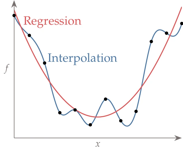
Figure 10.13:Interpolation models match the training data at the provided points, whereas regression models minimize the error between the training data and a function with an assumed trend.
Surrogate-based models can be based on interpolation or regression, as illustrated in Figure 10.13. Interpolation builds a function that exactly matches the provided training data. Regression models do not try to match the training data points exactly; instead, they minimize the error between a smooth trend function and the training data. The nature of the training data can help decide between these two types of surrogate models. Regression is particularly useful when the data are noisy. Interpolatory models may produce undesirable oscillations when fitting the noise. In contrast, regression models can find a smooth function that is less sensitive to the noise. Interpolation is useful when the data are highly multimodal (and not noisy). This is because a regression model may smooth over variations that are actually physical, whereas an interpolatory model can accurately capture those variations.
There are two main steps involved in either type of surrogate model. First, we select a set of basis functions, which represent the form for the model.
Second, we determine the model parameters that provide the best fit to the provided data. Determining the model parameters is an optimization problem, which we discuss first. We discuss linear regression and nonlinear regression, which are techniques for choosing model parameters for a given set of basis functions. Next, we discuss cross validation, which is a critical technique for selecting an appropriate model form. Finally, we discuss common basis functions.
10.3.1 Linear Least Squares Regression
A linear regression model does not mean that the surrogate is linear in the input variables but rather that the model is linear in its coefficients (i.e., linear in the parameters we are estimating). For example, the following equation is a two-dimensional linear regression model, where we use to represent our estimated model of the function :
This function is highly nonlinear, but it is classified as a linear regression model because the regression seeks to choose the appropriate values for the coefficients (and the function is linear in ).
A general linear regression model can be expressed as
where is a vector of weights, and is a vector of basis functions. In this section, we assume that the basis functions are provided. In general, the basis functions can be any set of functions that we choose (and typically they are nonlinear). It is usually desirable for these functions to be orthogonal.
The coefficients are chosen to minimize the error between our predicted function values and the actual function values . Because we want to minimize both positive and negative errors, we minimize the sum of the square of the errors (or a weighted sum of squared errors):[3]
The solution to this optimization problem is called a least squares solution. If the regression model is linear, we can simplify this objective and solve the problem analytically. Recall that , so the objective can be written as
We can express this in matrix form by defining the following:
The matrix is of size , where is the number of samples, the number of parameters in , and . This means that there should be more equations than unknowns or that we have sampled more points than the number of coefficients we need to estimate. This should make sense because our surrogate function is only an assumed form and generally not an exact fit to the actual underlying function. Thus, we need more data to create a good fit.
Then the optimization problem can be written in matrix form as:
Expanding the squared norm (i.e., ) gives
We can omit the last term from the objective because our optimization variables are , and the last term has no dependence:
This fits the general form for an unconstrained quadratic programming (QP) problem, as shown in Section 5.5.1:
where
Recall that an equality constrained QP (of which unconstrained is a subset) has an analytic solution as long as the QP is positive definite. In our case, we can show that is positive definite as long as is full rank:
This is not surprising because the objective is a sum of squared values. Referring back to the solution in Section 5.5.1, and removing the portions associated with the constraints, the solution is
In our case, this becomes
After simplifying, we have an analytic solution for the weights:
We sometimes express the linear relationship in Equation 10.12 as , although the case where there are more equations than unknowns does not typically have a solution (the problem is overdetermined). Instead, we seek the solution that minimizes the error , that is, Equation 10.23. The quantity is called the pseudoinverse of (or more specifically, the Moore–Penrose pseudoinverse), and thus we can write Equation 10.23 in the more compact form
This allows for a similar form to solving a linear system of equations where an inverse would be used instead. In solving both a linear system and the linear least-squares equation (Equation 10.23), we do not explicitly invert a matrix. For linear least squares, a QR factorization is commonly used for improved numerical conditioning as compared to solving Equation 10.23 directly.
A common variation of this approach is to use regularized least squares, which adds a term in the objective. The new objective is
where is a weight assigned to the second term. This second term attempts to reduce the magnitudes of the entries in while balancing the fit in the first term. This approach is particularly beneficial if the data contain strong outliers or are particularly noisy. The rationale for this approach is that we may want to accept a higher error (quantified by the first term) in exchange for smaller values for the coefficients. This generally leads to simpler, more generalizable models (e.g., by reducing the influence of some terms). A related extension uses a second term of the form . The idea is that we want a good fit, while maintaining parameters that are close to some known nominal values .
A regularized least squares problem can be solved with the same linear least squares approach. We can write the previous problem using concatenated matrices and vectors:
This is of the same linear form as before (), so we can reuse the solution (Equation 10.23):
For linear least squares (with or without regularization), we have seen that the optimization problem of determining the appropriate coefficients can be found analytically. We can also add linear constraints to the problem (equality or inequality), and the optimization remains a QP. In that case, the problem is still convex. Although it does not generally have an analytic solution, we can still quickly find the global optimum. This topic is discussed in Section 11.3.
10.3.2 Maximum Likelihood Interpretation
This section presents an alternative motivation for the sum of squared error approach used in the previous section. It is somewhat of a diversion from the present discussion, but it will be helpful in several results later in this chapter. In the previous section, we assumed linear models of the form
where we use for simplicity in writing instead of . The derivation remains the same for any arbitrary function of . The function is just a model, so we could say that it is equal to our actual observations plus an error term:
where captures the error associated with the data point. We assume that the error is normally distributed with mean zero and a standard deviation of :
The use of Gaussian uncertainty can be motivated by the central limit theorem, which states that for large sample sizes, the sum of random variables tends toward a Gaussian distribution regardless of the original distribution associated with each variable. In other words, the sample distribution of the sample mean is approximately Gaussian. Because we assume the error terms to be the sum of various random, independent perturbations, then by the central limit theorem, we expect the errors to be normally distributed.
We now substitute Equation 10.29 into Equation 10.30 to show the probability of conditioned on and parameterized by :
Once we include all the data points , we would like to compute the probability of observing conditioned on the inputs for a given set of parameters in . We call this the likelihood function . In this case, assuming all errors are independent, the total probability for observing the outputs is the product of the probability of observing each output:
Now we can pose this as an optimization problem where we wish to find the parameters that maximize the likelihood function; in other words, we maximize the probability that our model is consistent with the observed data. Because the objective is a product of multiple terms, it is helpful to take the logarithm of the objective. Maximizing or maximizing does not change the solution to the problem but makes it easier to solve. We call this the log likelihood function:
The first term has no dependence on , and so when optimizing ; it is just a scalar term that can be removed as follows:
Similarly, the denominator of the second term has no dependence on and is just a scalar that can also be removed:
Thus, maximizing the log likelihood function (maximizing the probability of observing the data) is equivalent to minimizing the sum of squared errors (the least-squares formulation). This derivation provides another motivation for using the sum of squared errors in regression.
10.3.3 Nonlinear Least Squares Regression
A surrogate model can be nonlinear in the coefficients. For example, building on the simple function shown earlier in Equation 10.9 we can add the coefficients and as follows:
The addition of and makes this function nonlinear in the coefficients. We can still estimate these parameters, but not analytically.
Equation 10.11 is still relevant; we still seek to minimize the sum of the squared errors:
For general nonlinear regression models, we cannot write a more specific form for as we could for the linear case, so we leave the objective as it is.
This is a nonlinear least-squares problem. The optimization problem is unconstrained, so any of the methods from Chapter 4 apply. We could also easily add constraints, for example, bounds on parameters, known relationships between parameters, and so forth, and use the methods from Chapter 5.
In contrast to the linear case, we need to provide a starting point, our best guess for the parameters, and we may need to deal with scaling, noise, multimodality, or any of the other potential challenges of general nonlinear optimization. Still, this is a relatively straightforward problem within the broader realm of engineering optimization problems.
Although the methods of Chapter 4 can be used if the problem remains unconstrained, there are more specialized methods available that take advantage of the specific structure of the problem. One popular approach to solving the nonlinear least-squares problem is the Levenberg–Marquardt algorithm, which we discuss in this section.
As a stepping stone towards the Levenberg–Marquardt algorithm, we first derive the Gauss–Newton algorithm, which is a modification of Newton’s method (Section 3.8) for solving nonlinear least-squares problems. One way to think of this algorithm is as an iterative linearization of the residual. Once it is linearized, we can apply the same methods we derived for linear least squares. We linearize the residual at iteration as
where is the step and the Jacobian is
After the linearization, the objective becomes
This is now the same form as linear least squares (Equation 10.14), so we can reuse its solution (Equation 10.23) to solve for the step
We now have an update formula for the coefficients at each iteration:
An alternative derivation for this formula is to consider a Newton step for an unconstrained optimizer. The objective is , and the formula for a Newton step (Section 4.4.3) is
The gradient is
or in matrix form:
The Hessian in index notation is
We can write it in matrix form as follows:
If we neglect the second term in the Hessian, then the Newton update is:
which is the same update as before.
Thus, another interpretation of this method is that a Gauss–Newton step is a modified Newton step where the second derivatives of the residual are neglected (and thus, a quasi-Newton approach to estimate second derivatives is not needed). This method is particularly effective near convergence because as (i.e., as we approach the solution to our residual minimization), the neglected term also approaches zero. The appeal of this approach is that we can often obtain an accurate prediction for the Hessian using only the first derivatives because of the known structure of the objective.
When the second term is not small, then the Gauss–Newton step may be too inaccurate. We could use a line search, but the Levenberg–Marquardt algorithm utilizes a different strategy. The idea is to regularize the problem as discussed in the previous section or, in other words, provide the ability to dampen the steps as needed. Each linearized subproblem becomes
Recall that the solution to this problem (see Equation 10.27) is
If , then we retain the Gauss–Newton step. Conversely, as becomes large, so that the is negligible, the step becomes
This is precisely the steepest-descent direction for our objective (see Equation 10.49), although with a small magnitude because is large. The parameter provides some control for directions ranging between Gauss–Newton and steepest descent.
The Levenberg–Marquardt algorithm has been revised to improve the scaling for components of the gradient that are small. The second minimization term weights all parameters equally. The scaling can be improved by multiplying by a diagonal matrix in the regularization as follows:
where is defined as
This matrix scales the objective by the diagonal elements of the Hessian. Thus, when is large, and the direction tends toward the steepest descent, the components of the gradient are scaled by the curvature, which reduces the amount of zigzagging.
The solution to the minimization problem of Equation 10.56 is
Finally, we describe one of the possible heuristics for selecting and updating the damping parameter . After a successful step (a sufficient reduction in the objective), is increased by a factor of . Conversely, an unsuccessful step is rejected, and is reduced by a factor ().
Rather than returning a scalar objective (), the user function should return a vector of the residuals because that vector is needed in the update steps (Equation 10.58). A potential convergence metric is a tolerance on objective value changes between subsequent iterations. The full procedure is described in Algorithm 10.3.
10.3.4 Cross Validation
The other important consideration for developing a surrogate model is the choice of the basis functions in . In some instances, we may know something about the model behavior and thus what type of basis functions should be used, but generally, the best way to determine the basis functions is through cross validation. Cross validation is also helpful in characterizing error, even if we already have a chosen set of basis functions. One of the reasons we use cross validation is to prevent overfitting. Overfitting occurs when we have too many degrees of freedom and closely fit a given set of data, but the resulting model has a poor predictive ability. In other words, we are fitting noise. The following example illustrates this idea with a one-dimensional function.
The solution to the overfitting problem highlighted in Example 10.5 is cross validation. Cross validation means that we use one set of data for training (creating the model) and a different set of data for assessing its predictive error. There are many different ways to perform cross validation; we describe two. Simple cross validation is illustrated in Figure 10.17 and consists of the following steps:
Randomly split your data into a training set and a validation set (e.g., a 70–30 split).
Train each candidate model (the different options for ) using only the training set, but evaluate the error with the validation set. The error on previously unseen data is called the generalization error ( in Figure 10.17).
Choose the model with the lowest generalization error, and optionally retrain that model using all of the data.
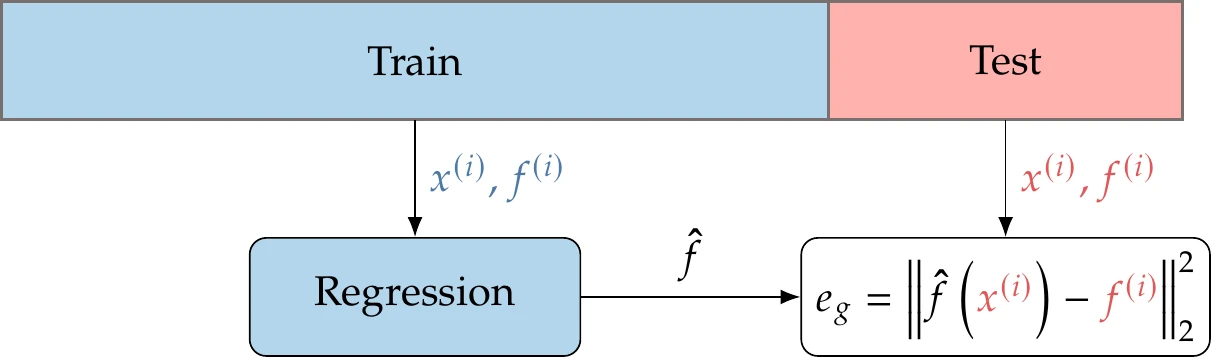
Figure 10.17:Simple cross-validation process.
An alternative option that is more involved but uses the data more effectively is called -fold cross validation. It is particularly advantageous when we have a small data set where we cannot afford to leave much out. This procedure is illustrated in Figure 10.18 and consists of the following steps:
Randomly split your data into sets (e.g., = 10).
Train each candidate model using the data from all sets except one (e.g., 9 of the 10 sets) and use the remaining set for validation. Repeat for all possible validation sets and average the performance.
Choose the model with the lowest average generalization error. Optionally, retrain with all the data.
The extreme version of this process, when training data are very limited, is leave-one-out cross validation (i.e., each testing subset consists of one data point).
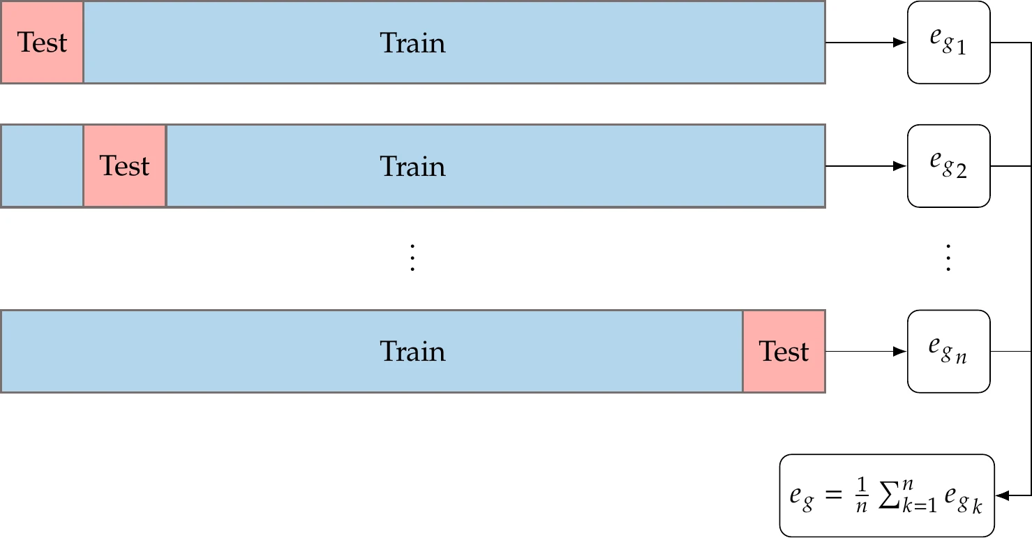
Figure 10.18:Diagram of -fold cross-validation process.
10.3.5 Common Basis Functions
Although cross validation can help us find the lowest generalization error among a provided set of basis functions, we still need to determine what sets of options to consider. This selection is crucial because our model is only as good as the available options, but increasing the number of options increases computational time. The possibilities for basis functions are as numerous as the types of function. As stated before, it is generally desirable that they form an orthogonal set. We focus on a few commonly used functions.
Polynomials
Polynomials, of which we have already seen a few examples, are useful in many applications. However, we typically use low-order polynomials for regression because high-order polynomials rarely generalize well. Polynomials can be particularly effective in cases where a knowledge of the physics suggests them to be an appropriate choice (e.g., drag varies quadratically with speed)
Because a lot of structure is already built into the model form, fewer data points are needed to create a reasonable model (e.g., a quadratic function in dimensions needs at least points, so this amounts to 6 points in two dimensions, 10 points in three dimensions, and so on).
Radial Basis Functions
Another common type of basis function is a radial basis function. Radial basis functions are functions that depend on the distance from some center point and can be written as follows:
where is the center point, and is the radius about the center point. Although the center points can be placed anywhere, we usually choose the sampling data as centering points:
This is often a useful choice because it captures the idea that our ability to predict function behavior is related to how close we are to known function values (in other words, nearby points are more highly correlated). This form naturally lends itself to interpolation, although regularization can be added to allow for regression. Polynomials are often combined with radial basis functions because the polynomial can capture global function behavior, while the radial basis functions can introduce modifications to capture local behavior.
One popular radial basis function is the Gaussian basis:
where are the model parameters. One of the forms of kriging discussed in the following section can be viewed as a radial basis function model with a Gaussian basis.
10.4 Kriging
Kriging is a popular surrogate modeling technique that can build approximations of highly nonlinear engineering simulations. We may not have a simple parametric form for such simulations that we can use with regression and expect a good fit.
Instead of tuning the parameters of a functional form that describes what the function is, kriging tunes the parameters of a statistical model that describes how the function behaves.
The kriging statistical model that approximates consists of two terms: a function that is meant to capture some of the function behavior and a random variable . Thus, we can write the kriging model as
When we evaluate the function we want to approximate at point , we get a scalar value . In contrast, when we evaluate the stochastic process (Equation 10.62) at , we get a random variable that has a normal distribution with mean and variance . Although we wrote as a function of , most kriging models consider this to be constant because the random variable term alone is effective in capturing the function behavior.
For the rest of this section, we discuss the case with constant , which is called ordinary kriging. Kriging is also referred to as Gaussian process interpolation, or more generally in the regression case discussed later in this section, as Gaussian process regression.
The power of the statistical model lies in how it treats the correlation between the random variables. Although we do not know the exact form of the error term , we can still make some reasonable assumptions about it. Consider two points in a sampling plan, and , and the corresponding terms, and . Intuitively, we expect to be close to whenever is close to . Therefore, it seems reasonable to assume that the correlation between and is a function of the distance between the two points.
In kriging, we assume that this correlation is given by a kernel function :
As a matrix, the kernel is represented as . Various kernel functions are used with kriging.[5]The most commonly used kernel function is
where , , and is the number of dimensions (i.e., the length of the vector ). If every , this becomes a Gaussian kernel.
Let us examine how the statistical model defined in Equation 10.62 captures the typical behavior of the function .
The parameter captures the typical value, and captures the expected variance. The kernel (or correlation) function (Equation 10.64) implicitly models continuous functions. If is continuous, we know that, as , then . This is captured in the kernel function because as , the correlation approaches 1. The parameter captures how active the function is in the th coordinate direction. A unit difference in variable () has a more significant impact on the correlation when is large. The exponent describes the smoothness of the function in the th coordinate direction. Values of close to 2 produce smooth functions, whereas values closer to zero produce functions with more variation.
Kriging surrogate modeling involves two main steps.
The first step consists of using the data to estimate the statistical model parameters , , , and . The second step consists of making predictions using the statistical model and these estimated parameter values.
The parameter estimation uses the same maximum likelihood approach from Section 10.3.2, but now it is more complicated. Let us denote the random variable as and the vector of random variables as , where is the number of samples. Similarly, and the vector of observed function values is . Using this notation, we can say that the vector is jointly normally distributed. This is also known as a multivariate Gaussian distribution.[6]The probability density function (PDF) (the likelihood that ) is
where is a vector of 1s with size , and is the determinant of the covariance,
The covariance between two elements and of is related to correlation by the following definition:[7]
We assume stationarity of the second moment, that is, the variance is constant in the domain.
The statistical model parameters and enter the likelihood (Equation 10.65) via their effect on the kernel (Equation 10.64) and hence on the covariance matrix (Equation 10.66).
We estimate the parameters using the maximum log likelihood approach from Section 10.3.2; that is, we maximize the probability of observing our data conditioned on the parameters and . Using a PDF (Equation 10.65) where is constant and the covariance is , yields the following likelihood function:
We now need to find the parameters , , , and that maximize this likelihood function, that is, maximize the probability of our observations .
As before, we take the logarithm to form the log likelihood function:
We can maximize part of this term analytically by taking derivatives with respect to and , setting them equal to zero, and solving for their optimal values to obtain:
We now substitute these values back into the log likelihood function (Equation 10.68), which yields
This function, also called the concentrated likelihood function, only depends on the kernel , which depends on and .
We cannot solve for optimal values of and analytically. Instead, we rely on numerical optimization to maximize Equation 10.71. Because can vary across a broad range, it is often better to search using logarithmic scaling. Once we solve that optimization problem, we compute the mean and variance in Equation 10.69 and Equation 10.70.
Now that we have a fitted model, we can make predictions at new points where we have not sampled. We do this by substituting into a formula called the kriging predictor. The formula is unique, but there are many ways to derive it.
One way to derive it is to find the function value at that is the most consistent with the behavior of the function captured by the fitted kriging model.
Let be our guess for the value of the function at . One way to assess the consistency of our guess is to add as an artificial point to our training data (so that we now have points) and estimate the likelihood using the parameters from our fitted kriging model. The likelihood of this augmented data can now be thought of as a function of : high values correspond to guessed values of that are consistent with function behavior captured by the fitted kriging model. Therefore, the value of that maximizes the likelihood of this augmented data set is a natural way to predict the value of the function. This is an optimization problem with a closed-form solution, and the corresponding formula is the kriging predictor.
Now we outline the derivation of the kriging predictor.[8]
With the augmented point, our function values are , where is the -vector of function values from the original training data. Then, the correlation matrix with the additional data point is
where is the correlation of the new point with the training data given by
The 1 in the bottom right of the augmented correlation matrix (Equation 10.72) is because the correlation of the new variable with itself is 1. The log likelihood function with these new augmented vectors and the previously determined parameters is as follows (see Equation 10.68):
We want to maximize this function with respect to . Because only the last term depends on (it is a part of ) we can omit the other terms and formulate the following:
This problem can be solved analytically, yielding the mean value of the kriging prediction,
The mean square error of the kriging prediction (that is, the expected squared value of the error) is given by[9]
One attractive feature of kriging models is that they are interpolatory and thus match the training data exactly. To see how this is true, if is the same as one of the training data points, , then is just th column of . Hence, is a vector , with all zeros except for 1 in the th element. In the prediction (Equation 10.75), and so the last term is , which means that .
In the mean square error (Equation 10.76), is the same as . This is the th element of , which is 1. Therefore, the first two terms in the brackets in Equation 10.76 cancel, and the last term is zero, yielding . This is expected; if we already sampled the point, the uncertainty about its function value should be zero.
When describing a fitted kriging model, we often refer to the standard error as the square root of this quantity (i.e., ). The standard error is directly related to the confidence interval (e.g., standard error corresponds to a 68 percent confidence interval).
If we can provide the gradients of the function at the training data points (in addition to the function values), we can use that information to build a more accurate kriging model. This approach is called gradient-enhanced kriging (GEK). The methodology is the same as before, except we add more observed outputs (i.e., in addition to the function values at the sampled points, we add their gradients). In addition to considering the correlation between the function values at different sampled points, the kernel matrix needs to be expanded to consider correlations between function values and gradients, gradients and function values, and among gradient components.
We can use still use equation (Equation 10.75) for the GEK predictor and equation (Equation 10.76) for the mean square error if we plug in “expanded versions” of the outputs , the vector , the matrix , and the vector of 1s, .
We expand the output vector to include not just the function values at the sampled points but also their gradients:
This vector is of length , where is the dimension of . The gradients are usually provided at the same locations as the function samples, but that is not required.
Recall that the term in Equation 10.75 for the kriging predictor represents the expected value of the random variables . Now that we have expanded the outputs to include the gradients at the sampled points, the mean vector needs to be expanded to include the expected values of , which are all zero.
We can still use in the formula for the predictor if we use the following definition:
where 1 occurs for the first entries, and 0 for the remaining entries.
The additional correlations (between function values and derivatives and between the derivatives themselves) are as follows:
Here, we use and to represent a component of a vector, and we use as shorthand. For our particular kernel choice (Equation 10.64), these correlations become the following:
where we used . Putting this all together yields the expanded correlation matrix:
where the block representing the first derivatives is
and the matrix of second derivatives is
We can still get the estimates and with Equation 10.69 and Equation 10.70 using the expanded versions of , , and replacing in Equation 10.76 with , which is the new length of the outputs.
The predictor equations (Equation 10.75 and Equation 10.76) also apply with the expanded matrices and vectors. However, we also need to expand in these computations to include the correlations between the gradients at the sampled points with the gradient at the point where we make a prediction. Thus, the expanded is:
One difficulty with GEK is that the kernel matrix quickly grows in size as the dimension of the problem increases, the number of samples increases, or both. Various approaches have been proposed to improve the scaling with higher dimensions, such as a weighted sum of smaller correlation matrices9 or a partial least squares approach.6
The version of kriging in this section is interpolatory. For noisy data, a regression approach can be used by modifying the correlation matrix as follows:
with . This adds a positive constant along the diagonal, so the model no longer correlates perfectly with the provided points. The parameter is then an additional parameter to estimate in the maximum likelihood optimization. Even for interpolatory models, this term is often still added to the covariance matrix with a small constant value of (near machine precision) to ensure that the correlation matrix is invertible. This section focused on the most common choices when using kriging, but many other versions exist.10
10.5 Deep Neural Networks
Like kriging, deep neural nets can be used to approximate highly nonlinear simulations where we do not need to provide a parametric form. Neural networks follow the same basic steps described for other surrogate models but with a unique model leading to specialized approaches for derivative computation and optimization strategy. Neural networks loosely mimic the brain, which consists of a vast network of neurons. In neural networks, each neuron is a node that represents a simple function. A network defines chains of these simple functions to obtain composite functions that are much more complex. For example, three simple functions, , and , may be chained into the composite function (or network):
Even though each function may be simple, the composite function can express complex behavior. Most neural networks are feedforward networks, meaning that information flows from inputs to outputs . Recurrent neural networks include feedback connections.
Figure 10.24 shows a diagram of a neural network. Each node represents a neuron. The neurons are connected between consecutive layers, forming a dense network. The first layer is the input layer, the last one is the output layer, and the middle ones are the hidden layers. The total number of layers is called the network’s depth. Deep neural networks have many layers, enabling the modeling of complex behavior.
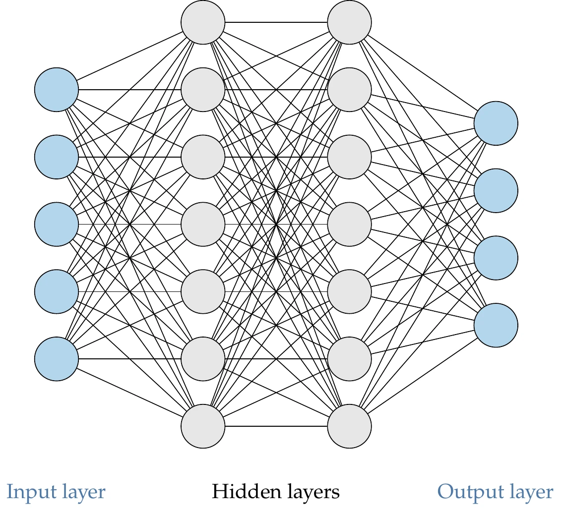
Figure 10.24:Deep neural network with two hidden layers.
The first and last layers can be viewed as the inputs and outputs of a surrogate model. Each neuron in the hidden layer represents a function. This means that the output from a neuron is a number, and thus the output from a whole layer can be represented as a vector . We represent the vector of values for layer by , and the value for the th neuron in layer by .
Consider a neuron in layer . This neuron is connected to many neurons from the previous layer (see the first part of Figure 10.25). We need to choose a functional form for each neuron in the layer that takes in the values from the previous layer as inputs. Chaining together linear functions would yield another linear function. Therefore, some layers must use nonlinear functions.
The most common choice for hidden layers is a layer of linear functions followed by a layer of functions that create nonlinearity. A neuron in the linear layer produces the following intermediate variable:
In vector form:
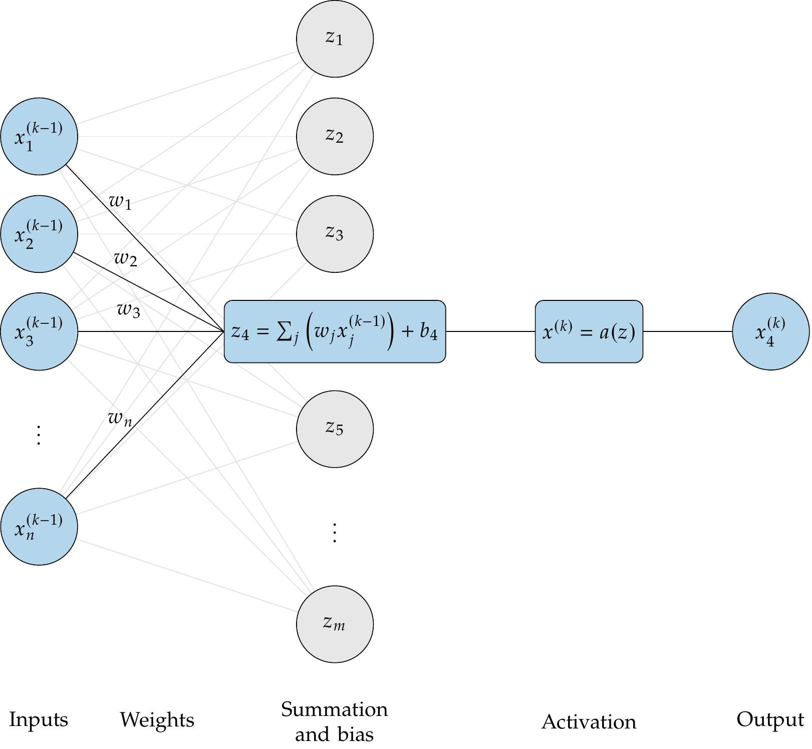
Figure 10.25:Typical functional form for a neuron in the neural net.
The first term is a weighted sum of the values from the neurons in the previous layer. The vector contains the weights. The term is the bias, which is an offset that scales the significance of the overall output. These two terms are analogous to the weights used in the previous section but with the constant term separated for convenience. The second column of Figure 10.25 illustrates the linear (summation and bias) layer.
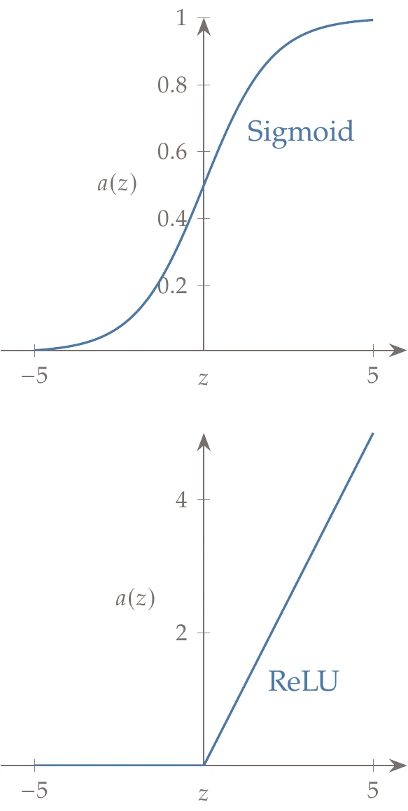
Figure 10.26:Activation functions.
Next, we pass through an activation function, which we call .
Historically, one of the most common activation functions has been the sigmoid function:
This function is shown in the top plot of Figure 10.26. The sigmoid function produces values between 0 and 1, so large negative inputs result in insignificant outputs (close to 0), and large positive inputs produce outputs close to 1.
Most modern neural nets use a rectified linear unit (ReLU) as the activation function:
This function is shown in the bottom plot of Figure 10.26. The ReLU has been found to be far more effective than the sigmoid function in producing accurate neural nets. This activation function eliminates negative inputs. Thus, the bias term can be thought of as a threshold establishing what constitutes a significant value. The final two columns of Figure 10.25 illustrate the activation step.
Combining the linear function with the activation function produces the output for the neuron:
To compute the outputs for all the neurons in this layer, the weights for one neuron form one row in a matrix of weights and we can write:
or
The activation function is applied separately for each row. The following equation is more explicit (where is the row of ):
This neural net is now parameterized by a number of weights. Like other surrogate models, we need to determine the optimal value for these parameters (i.e., train the network) using training data. In the example of Figure 10.24, there is a layer of 5 neurons, 7 neurons, 7 neurons, and then 4 neurons, and so there would be weights and bias terms, giving a total of 130 variables. This represents a small neural net because there are few inputs and few outputs. Large neural nets can have millions of variables. We need to optimize those variables to minimize a cost function.
As before, we use a maximum likelihood estimate where we optimize the parameters (weights and biases in this case) to maximize the probability of observing the output data conditioned on our inputs . As shown in Section 10.3.2, this results in a sum of squared errors function:
We now have the objective and variables in place to train the neural net. As with the other models discussed in this chapter, it is critical to set aside some data for cross validation.
Because the optimization problem (Equation 10.95) often has a large number of parameters , we generally use a gradient-based optimization algorithm (however the algorithms of Chapter 4 are modified as we will discuss shortly). To solve Equation 10.95 using gradient-based optimization, we require the derivatives of the objective function with respect to the weighs . Because the objective is a scalar and the number of weights is large, reverse-mode algorithmic differentiation (AD) (see Section 6.6) is ideal to compute the required derivatives.
Reverse-mode AD is known in the machine learning community as backpropagation.[10] Whereas general-purpose reverse-mode AD operates at the code level, backpropagation usually operates on larger sets of operations and data structures defined in machine learning libraries. Although less general, this approach can increase efficiency and stability.
The ReLU activation function (Figure 10.26, bottom) is not differentiable at , but in practice, this is generally not problematic—primarily because these methods typically rely on inexact gradients anyway, as discussed next.
The objective function in Equation 10.95 consists of a sum of subfunctions, each of which depends on a single data point (. Objective functions vary across machine learning applications, but most have this same form:
where
As previously mentioned, the challenge with these problems is that we often have large training sets where may be in the billions. That means that computing the objective can be costly, and computing the gradient can be even more costly.
If we divide the objective by (which does not change the solution), the objective function becomes an approximation of the expected value (see Section A.9):
From probability theory, we know that we can estimate an expected value from a smaller set of random samples. For the application of estimating a gradient, we call this subset of random samples a minibatch , where is usually between 1 and a few hundred. The entries do not correspond to the first entries but are drawn randomly from a uniform probability distribution (Figure 10.27). Using the minibatch, we can estimate the gradient as the sum of the subfunction gradients at different training points:
Thus, we divide the training data into these minibatches and use a new minibatch to estimate the gradients at each iteration in the optimization.
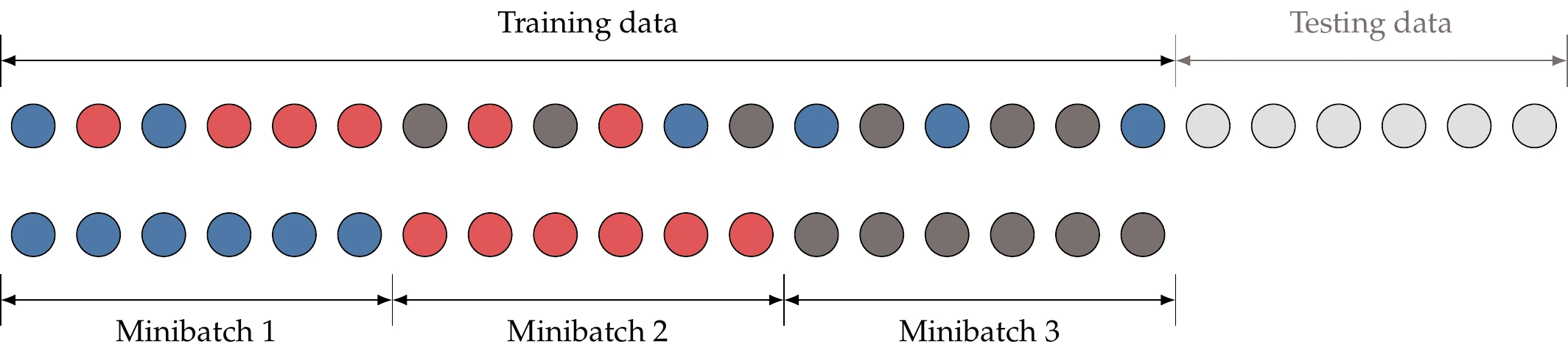
Figure 10.27:Minibatches are randomly drawn from the training data.
This approach works well for these specific problems because of the unique form for the objective (Equation 10.98). As an example, for one million training samples, a single gradient evaluation would require evaluating all one million training samples. Alternatively, for a similar cost, a minibatch approach can update the optimization variables a million times using the gradient estimated from one training sample at a time. This latter process usually converges much faster, mainly because we are only fitting parameters against limited data in these problems, so we generally do not need to find the exact minimum.
Typically, this gradient is used with steepest descent methods (Section 4.4.1), more typically referred to as gradient descent in the machine learning communities. As discussed in Chapter 4, steepest descent is not the most effective optimization algorithm. However, steepest descent with the minibatch updates, called stochastic gradient descent, has been found to work well in machine learning applications. This suitability is primarily because (1) many machine learning optimizations are performed repeatedly, (2) the true objective is difficult to formalize, and (3) finding the absolute minimum is not as important as finding a good enough solution quickly. One key difference in stochastic gradient descent relative to the steepest descent method is that we do not perform a line search. Instead, the step size (called the learning rate in machine learning applications) is a preselected value that is usually decreased between major optimization iterations.
Stochastic minibatching is easily applied to first-order methods and has thus driven the development of improvements on stochastic gradient descent, such as momentum, Adagrad, and Adam.12 Although some of these methods may seem somewhat ad hoc, there is mathematical rigor to many of them.13 Batching makes the gradients noisy, so second-order methods are generally not pursued. However, ongoing research is exploring stochastic batch approaches that might effectively leverage the benefits of second-order methods.
10.6 Optimization and Infill
Once a surrogate model has been built, optimization may be performed using the surrogate function values. That is, instead of minimizing the expensive function , we minimize the model , as previously illustrated in Figure 10.1.
The surrogate model may be static, but more commonly, it is updated between optimization iterations by adding new training data and rebuilding the model.
The process by which we select new data points is called infill. There are two main approaches to infill: prediction-based exploitation and error-based exploration. Typically, only one infill point is chosen at a time. The assumption is that evaluating the model is computationally expensive, but rebuilding and evaluating the surrogate is cheap.
10.6.1 Exploitation
For models that do not provide uncertainty estimates, the only real option is exploitation. A prediction-based exploitation infill strategy adds an infill point wherever the surrogate predicts the optimum. The reasoning behind this approach is that in SBO, we do not necessarily care about having a globally accurate surrogate; instead, we only care about having an accurate surrogate near the optimum.
The most logical point to sample is thus the optimum predicted by the surrogate. Likely, the location predicted by the surrogate will not be at the true optimum. However, evaluating this point adds valuable information in the region of interest.
We rebuild the surrogate and re-optimize, repeating the process until convergence. This approach usually results in the quickest convergence to an optimum, which is desirable when the actual function is expensive to evaluate. The downside is that we may converge prematurely to an inferior local optimum for problems with multiple local optima.
Even though the approach is called exploitation, the optimizer used on the surrogate can be a global search method (gradient-based or gradient-free), although it is usually a local search method. If uncertainty is present, using the mean value of the surrogate as the infill criteria results in essentially an exploitation strategy.
The algorithm is outlined in Algorithm 10.4. Convergence could be based on a maximum number of iterations or a tolerance for the objective function’s fractional change.
10.6.2 Efficient Global Optimization
An alternative approach to infill uses error-based exploration. This approach requires using kriging (Section 10.4) or another surrogate approach that predicts not just function values but also error estimates. Although many infill metrics exist within this category, we focus on a popular one called expected improvement, and the associated algorithm, efficient global optimization (EGO).14
As stated previously, sampling where the mean is low is an exploitation strategy, but we do not necessarily want to sample where the uncertainty is high. That may lead to wasteful function calls in regions of the design space where the surrogate model is inaccurate but which are far from any optimum. In effect, this strategy would be like a larger sampling plan aiming to reduce error everywhere in the surrogate. Instead, we want to sample where we have the maximum probability of finding a better point.
Let the best solution we have found so far be . The improvement for any new test point is then given by
If , there is no improvement, but if , the improvement is positive. However, is not a deterministic value in this model but rather a probability distribution. Thus, the expected improvement is the expected value (or mean) of the improvement:
The expected value for a kriging model can be found analytically as:
where and are the CDF and PDF, respectively, for the standard normal distribution, and and are the mean and standard error functions produced from kriging ( Equation 10.75 and Equation 10.76).
The algorithm is similar to that of the previous section (Algorithm 10.4), but instead of choosing the minimum of the surrogate, the selected infill point is the point with the greatest expected improvement. The corresponding algorithm is detailed in Algorithm 10.5.
10.7 Summary
Surrogate-based optimization can be an effective approach to optimization problems where models are expensive to evaluate or noisy.
The first step in building a surrogate model is sampling, in which we select the points that are evaluated to obtain the training data. Full factorial searches are too expensive for even a modest number of variables, and random sampling does not provide good coverage, so we need techniques that provide good coverage with a small number of samples. Popular techniques for this kind of sampling include LHS and low-discrepancy sequences.
The next step is surrogate selection and construction. For a given choice of basis functions, regression is used to select optimal model parameters. Cross validation is a critical component of this process. We want good predictive capability, which means that the models work well on data that the model has not been trained against. Model selection often involves trade-offs of more rigid models that do not need as much training data versus more flexible models that require more training data. Polynomials are often used for regression problems because a relatively small number of samples can be used to capture model behavior. Radial basis functions are more often used for interpolation because they can handle multimodal behavior but may require more training data.
Kriging and deep neural nets are two options that model more complex and multimodal design spaces. When using these models, special considerations are needed for efficiency, such as using symmetric matrix factorizations and gradients for kriging and using backpropagation and stochastic gradients for deep neural nets.
The last step of the process is infill, where points are sampled during optimization to update the surrogate model. Some approaches are exploitation-based, where we perform optimization using the surrogate and then use the optimal solution to update the model. Other approaches are exploration-based, where we sample not just at the deterministic optimum but also at points where the expected improvement is high. Exploration-based approaches require surrogate models that provide uncertainty estimates, such as kriging models.
Problems
Nonlinear least squares. Implement a Levenberg–Marquardt algorithm and demonstrate its performance on the Rosenbrock function from three different starting points.
Kriging. Implement kriging (without gradients) and demonstrate its fit on the following one-dimensional function:
where , using the following five sample points: .
Efficient global optimization. Use EGO with the function from the previous problem, showing the iteration history until the expected improvement reduces below 0.001.
PDFs and CDFs are reviewed in Section A.9.
A set of numbers is pairwise prime if there is no positive integer that can evenly divide any pair of them, except 1. Typically, though, we just use the first prime numbers.
The choice of minimizing the sum of the squares rather than the sum of the absolute values or some other metric is not arbitrary. The motivation for using the sum of the squares is discussed further in the following section.
Kernel functions must be symmetric and positive definite because a covariance matrix is always symmetric and positive definite.
There are other ways to derive kriging that do not require making assumptions on the random variable distribution type.
Covariance and correlation are briefly reviewed in Section A.9.
- Faure, H. (1982). Discrépance des suites associées à un systéme de numération (en dimension s). Acta Arithmetica, 41, 337–351. 10.4064/aa-41-4-337-351
- Faure, H., & Lemieux, C. (2009). Generalized Halton sequences in 2008: A comparative study. ACM Transactions on Modeling and Computer Simulation, 19(4), 1–31. 10.1145/1596519.1596520
- Sobol, I. M. (1967). On the distribution of points in a cube and the approximate evaluation of integrals. USSR Computational Mathematics and Mathematical Physics, 7(4), 86–112. 10.1016/0041-5553(67)90144-9
- Niederreiter, H. (1988). Low-discrepancy and low-dispersion sequences. Journal of Number Theory, 30(1), 51–70. 10.1016/0022-314X(88)90025-X
- Bouhlel, M. A., Hwang, J. T., Bartoli, N., Lafage, R., Morlier, J., & Martins, J. R. R. A. (2019). A Python surrogate modeling framework with derivatives. Advances in Engineering Software, 102662. https://doi.org/10.1016/j.advengsoft.2019.03.005
- Bouhlel, M. A., & Martins, J. R. R. A. (2019). Gradient-enhanced kriging for high-dimensional problems. Engineering with Computers, 1(35), 157–173. 10.1007/s00366-018-0590-x
- Jones, D. R. (2001). A taxonomy of global optimization methods based on response surfaces. Journal of Global Optimization, 21, 345–383. 10.1023/A:1012771025575
- Sacks, J., Welch, W. J., Mitchell, T. J., & Wynn, H. P. (1989). Design and analysis of computer experiments. Statistical Science, 4(4), 409–423. 10.2307/2245858
- Han, Z.-H., Zhang, Y., Song, C.-X., & Zhang, K.-S. (2017). Weighted gradient-enhanced kriging for high-dimensional surrogate modeling and design optimization. AIAA Journal, 55(12), 4330–4346. 10.2514/1.J055842
- Forrester, A., Sobester, A., & Keane, A. (2008). Engineering Design via Surrogate Modelling: A Practical Guide. John Wiley & Sons.
- Baydin, A. G., Pearlmutter, B. A., Radul, A. A., & Siskind, J. M. (2018). Automatic differentiation in machine learning: A survey. Journal of Machine Learning Research, 18(1), 5595–5637. 10.5555/3122009.3242010
- Ruder, S. (2016). An overview of gradient descent optimization algorithms. In CoRR: Vol. abs/1609.04747. http://arxiv.org/abs/1609.04747
- Goh, G. (2017). Why momentum really works. Distill. 10.23915/distill.00006
- Jones, D. R., Schonlau, M., & Welch, W. J. (1998). Efficient global optimization of expensive black-box functions. Journal of Global Optimization, 13, 455–492. 10.1023/A:1008306431147