Multiobjective Optimization - Engineering Design Optimization

Up to this point in the book, all of our optimization problem formulations have had a single objective function. In this chapter, we consider multiobjective optimization problems, that is, problems whose formulations have more than one objective function. Some common examples of multiobjective optimization include risk versus reward, profit versus environmental impact, acquisition cost versus operating cost, and drag versus noise.

9.1 Multiple Objectives¶

Before discussing how to solve multiobjective problems, we must first explore what it means to have more than one objective. In some sense, there is no such thing as a multiobjective optimization problem. Although many metrics are important to the engineer, only one thing can be made best at a time. A common technique when presented with multiple objectives is to assign weights to the various objectives and combine them into a single objective.

More generally, multiobjective optimization helps explore the trade-offs between different metrics. Still, if we select one design from the presented options, we have indirectly chosen a single objective. However, the corresponding objective function may be difficult to formulate beforehand.

Example 9.1 (Selecting an objective)

Determining the appropriate objective is often a real challenge. For example, in designing an aircraft, we may decide that minimizing drag and minimizing weight are important. However, these metrics compete with each other and cannot be minimized simultaneously. Instead, we may conclude that maximizing range (the distance the aircraft can fly) is the underlying metric that matters most for our application and appropriately balances the trade-offs between weight and drag. Or perhaps maximizing range is not the right metric. Range may be important, but only insofar as we reach some threshold. Increasing the range does not increase the value because the range is a constraint. The underlying objective in this scenario may be some other metric, such as operating costs.

Despite these considerations, there are still good reasons to pursue a multiobjective problem. A few of the most common reasons are as follows:

Multiobjective optimization can quantify the trade-off between different objectives. The benefits of this approach will become apparent when we discuss Pareto surfaces and can lead to important design insights.
Multiobjective optimization provides a “family” of designs rather than a single design. A family of options is desirable when decision-making needs to be deferred to a later stage as more information is gathered. For example, an executive team or higher-fidelity numerical simulations may be used to make later design decisions.
For some problems, the underlying objective is either unknown or too difficult to compute. For example, cost and environmental impact may be two important metrics for a new design. Although the latter could arguably be turned into a cost, doing so may be too difficult to quantify and add an unacceptable amount of uncertainty (see Chapter 12).

Mathematically, the only change to our optimization problem formulation is that the objective statement,

\begin{align} \underset{x}{\text{minimize}} &\quad f(x) \, , \end{align}

(9.1)

becomes

\underset{x}{\text{minimize}} \quad f(x) = \begin{bmatrix}f_1(x)\\f_2(x)\\ \vdots\\f_{n_f}(x)\end{bmatrix}, \quad \text{where} \quad n_f \ge 2 \, .

(9.2)

The constraints are unchanged unless some of them have been reformulated as objectives. This multiobjective formulation might require trade-offs when trying to minimize all functions simultaneously because, beyond some point, further reduction in one objective can only be achieved by increasing one or more of the other objectives.

One exception occurs if the objectives are independent because they depend on different sets of design variables. Then, the objectives are said to be separable, and they can be minimized independently. If there are constraints, these need to be separable as well. However, separable objectives and constraints are rare because functions tend to be linked in engineering systems.

Given that multiobjective optimization requires trade-offs, we need a new definition of optimality. In the next section, we explain how there is an infinite number of optimal points, forming a surface in the space of objective functions. After defining optimality for multiple objectives, we present several possible methods for solving multiobjective optimization problems.

9.2 Pareto Optimality¶

With multiple objectives, we have to reconsider what it means for a point to be optimal. In multiobjective optimization, we use the concept of Pareto optimality.

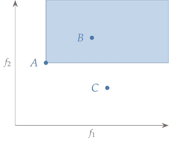
Three designs, A, B, and C, are plotted against two objectives, f_1 and f_2. The region in the shaded rectangle highlights points that are dominated by design A. — Figure 9.1:Three designs, $A$ , $B$ , and $C$ , are plotted against two objectives, $f_1$ and $f_2$ . The region in the shaded rectangle highlights points that are dominated by design $A$ .

Figure 9.1 shows three designs measured against two objectives that we want to minimize: $f_1$ and $f_2$ . Let us first compare design A with design B. From the figure, we see that design A is better than design B in both objectives. In the language of multiobjective optimization, we say that design A dominates design B. One design is said to dominate another design if it is superior in all objectives (design A dominates any design in the shaded rectangle). Comparing design A with design C, we note that design A is better in one objective ( $f_1$ ) but worse in the other objective ( $f_2$ ). Neither design dominates the other.

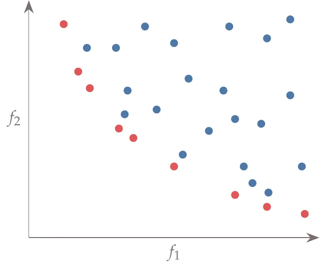
A plot of all the evaluated points in the design space plotted against two objectives, f_1 and f_2. The set of red points is not dominated by any other and is thus the current approximation of the Pareto set. — Figure 9.2:A plot of all the evaluated points in the design space plotted against two objectives, $f_1$ and $f_2$ . The set of red points is not dominated by any other and is thus the current approximation of the Pareto set.

A point is said to be nondominated if none of the other evaluated points dominate it (Figure 9.2). If a point is nondominated by any point in the entire domain, then that point is called Pareto optimal. This does not imply that this point dominates all other points; it simply means no other point dominates it. The set of all Pareto optimal points is called the Pareto set. The Pareto set refers to the vector of points $x^*$ , whereas the Pareto front refers to the vector of functions $f(x^*)$ .

Example 9.2 (A Pareto front in wind farm optimization)

The Pareto front is a valuable tool to produce design insights. Figure 9.3 shows a notional Pareto front for a wind farm optimization. The two objectives are maximizing power production (shown with a negative sign so that it is minimized) and minimizing noise.

Figure 9.3:A notional Pareto front representing power and noise trade-offs for a wind farm optimization problem.

The Pareto front is helpful to understand trade-off sensitivities. For example, the left endpoint represents the maximum power solution, and the right endpoint represents the minimum noise solution. The nature of the curve on the left side tells us how much power we have to sacrifice for a given reduction in noise. If the slope is steep, as is the case in the figure, we can see that a small sacrifice in maximum power production can be exchanged for significantly reduced noise. However, if more significant noise reductions are sought, then large power reductions are required. Conversely, if the left side of the figure had a flatter slope, we would know that small reductions in noise would require significant decreases in power. Understanding the magnitude of these trade-off sensitivities helps make high-level design decisions.

9.3 Solution Methods¶

Various solution methods exist for solving multiobjective problems. This chapter does not cover all methods but highlights some of the more commonly used approaches. These include the weighted-sum method, the epsilon-constraint method, the normal boundary intersection (NBI) method, and evolutionary algorithms.

9.3.1 Weighted Sum¶

The weighted-sum method is easy to use, but it is not particularly efficient. Other methods exist that are just as simple but have better performance. It is only introduced because it is well known and is frequently used. The idea is to combine all of the objectives into one objective using a weighted sum, which can be written as

\bar f(x) = \sum_{i=1}^{n_f} w_i f_i(x) \, ,

(9.3)

where $n_f$ is the number of objectives, and the weights are usually normalized such that

\sum_{i=1}^{n_f} w_i = 1 \, .

(9.4)

If we have two objectives, the objective reduces to

\bar f(x) = w f_1(x) + (1 - w) f_2(x) \, ,

(9.5)

where $w$ is a weight in $[0, 1]$ .

Consider a two-objective case. Points on the Pareto set are determined by choosing a weight $w$ , completing the optimization for the composite objective, and then repeating the process for a new value of $w$ . It is straightforward to see that at the extremes $w = 0$ and $w = 1$ , the optimization returns the designs that optimize one objective while ignoring the other. The weighted-sum objective forms an equation for a line with the objectives as the ordinates.

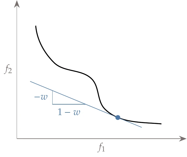
The weighted-sum method defines a line for each value of w and finds the point tangent to the Pareto front. — Figure 9.4:The weighted-sum method defines a line for each value of $w$ and finds the point tangent to the Pareto front.

Conceptually, we can think of this method as choosing a slope for the line (by selecting $w$ ), then pushing that line down and to the left as far as possible until it is just tangent to the Pareto front (Figure 9.4). With this form of the objective, the slope of the line would be

\frac{df_2}{df_1}= \frac{-w}{1-w} \, .

(9.6)

This procedure identifies one point in the Pareto set, and the procedure must then be repeated with a new slope.

The main benefit of this method is that it is easy to use.

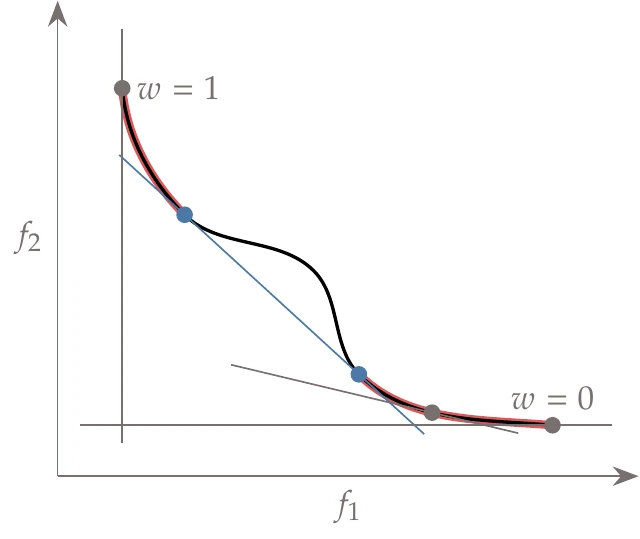
Figure 9.5:The convex portions of this Pareto front are the portions highlighted.

However, the drawbacks are that (1) uniform spacing in $w$ leads to nonuniform spacing along with the Pareto set, (2) it is not apparent which values of $w$ should be used to sweep out the Pareto set evenly, and (3) this method can only return points on the convex portion of the Pareto front.

In Figure 9.5, we highlight the convex portions of the Pareto front from Figure 9.4. If we utilize the concept of pushing a line down and to the left, we see that these are the only portions of the Pareto front that can be found using a weighted-sum method.

9.3.2 Epsilon-Constraint Method¶

The epsilon-constraint method works by minimizing one objective while setting all other objectives as additional constraints:1

\begin{aligned} \underset{x}{\text{minimize}} &\quad f_i\\ \text{subject to} &\quad f_j \le \varepsilon_j \quad \text{for all } j \neq i \\ &\quad g(x) \le 0 \\ &\quad h(x) = 0 \, . \end{aligned}

(9.7)

Then, we must repeat this procedure for different values of $\varepsilon_j$ .

This method is visualized in Figure 9.6. In this example, we constrain $f_1$ to be less than or equal to a certain value and minimize $f_2$ to find the corresponding point on the Pareto front. We then repeat this procedure for different values of $\varepsilon$ .

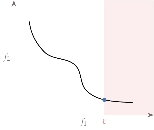
The vertical line represents an upper bound constraint on f_1. The other objective, f_2, is minimized to reveal one point in the Pareto set. This procedure is then repeated for different constraints on f_1 to sweep out the Pareto set. — Figure 9.6:The vertical line represents an upper bound constraint on $f_1$ . The other objective, $f_2$ , is minimized to reveal one point in the Pareto set. This procedure is then repeated for different constraints on $f_1$ to sweep out the Pareto set.

One advantage of this method is that the values of $\varepsilon$ correspond directly to the magnitude of one of the objectives, so determining appropriate values for $\varepsilon$ is more intuitive than selecting the weights in the previous method. However, we must be careful to choose values that result in a feasible problem. Another advantage is that this method reveals the nonconvex portions of the Pareto front. Both of these reasons strongly favor using the epsilon-constraint method over the weighted-sum method, especially because this method is not much harder to use. Its main limitation is that, like the weighted-sum method, a uniform spacing in $\varepsilon$ does not generally yield a uniform spacing of the Pareto front (though it is usually much better spaced than weighted-sum), and therefore it might still be inefficient, particularly with more than two objectives.

9.3.3 Normal Boundary Intersection¶

The NBI method is designed to address the issue of nonuniform spacing along the Pareto front.2 We first find the extremes of the Pareto set; in other words, we minimize the objectives one at a time. These extreme points are referred to as anchor points. Next, we construct a plane that passes through the anchor points. We space points along this plane (usually evenly) and, starting from those points, solve optimization problems that search along directions normal to this plane.

This procedure is shown in Figure 9.7 for a two-objective case. In this case, the plane that passes through the anchor points is a line. We now space points along this line by choosing a vector of weights $b$ , as illustrated on the left-hand of Figure 9.7. The weights are constrained such that $b_i \in [0, 1]$ , and $\sum_i b_i = 1$ . If we make $b_i = 1$ and all other entries zero, then this equation returns one of the anchor points, $f(x_i^*)$ . For two objectives, we would set $b = [w, 1-w]$ and vary $w$ in equal steps between 0 and 1.

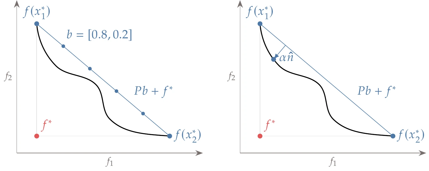
Figure 9.7:A notional example of the NBI method. A plane is created that passes through the single-objective optima (the anchor points), and solutions are sought normal to that plane for a more evenly spaced Pareto front.

Starting with a specific value of $b$ , we search along a direction perpendicular to the line defined by the anchor points, represented by $\alpha \hat n$ in Figure 9.7 (right). We seek to find the point along this direction that is the farthest away from the anchor points line (a maximization problem), with the constraint that the point is consistent with the objective functions. The resulting optimal point found along this direction is a point on the Pareto front. We then repeat this process for another set of weighting parameters in $b$ .

We can see how this method is similar to the epsilon-constraint method, but instead of searching along lines parallel to one of the axes, we search along lines perpendicular to the plane defined by the anchor points. The idea is that even spacing along this plane is more likely to lead to even spacing along the Pareto front.

Mathematically, we start by determining the anchor points, which are just single-objective optimization problems. From the anchor points, we define what is called the utopia point. The utopia point is an ideal point that cannot be obtained, where every objective reaches its minimum simultaneously (shown in the lower-left corner of Figure 9.7):

f^* = \begin{bmatrix} f_1(x_1^*)\\ f_2(x_2^*)\\ \vdots\\ f_n(x_n^*) \end{bmatrix} \, ,

(9.8)

where $x_i^*$ denotes the design variables that minimize objective $f_i$ . The utopia point defines the equation of a plane that passes through all anchor points,

P b + f^* \, ,

(9.9)

where the $i{\text{th}}$ column of $P$ is $f(x_i^*) - f^*$ . A single vector $b$ , whose length is given by the number of objectives, defines a point on the plane.

We now define a vector ( $\hat{n}$ ) that is normal to this plane, in the direction toward the origin. We search along this vector using a step length $\alpha$ , while maintaining consistency with our objective functions $f(x)$ yielding

f(x) = P b + f^* + \alpha \hat{n} \, .

(9.10)

Computing the exact normal ( $\hat{n}$ ) is involved, and the vector does not need to be exactly normal. As long as the vector points toward the Pareto front, then it will still yield well-spaced points. In practice, a quasi-normal vector is often used, such as,

\tilde{n} = -P e \, ,

(9.11)

where $e$ is a vector of 1s.

We now solve the following optimization problem, for a given vector $b$ , to yield a point on the Pareto front:

\begin{aligned} \underset{x, \alpha}{\text{maximize}} &\quad \alpha\\ \text{subject to} &\quad P b + f^* + \alpha \hat{n} = f(x)\\ &\quad g(x) \le 0\\ &\quad h(x) = 0 \, . \end{aligned}

(9.12)

This means that we find the point farthest away from the anchor-point plane, starting from a given value for $b$ , while satisfying the original problem constraints. The process is then repeated for additional values of $b$ to sweep out the Pareto front.

In contrast to the previously mentioned methods, this method yields a more uniformly spaced Pareto front, which is desirable for computational efficiency, albeit at the cost of a more complex methodology.

For most multiobjective design problems, additional complexity beyond the NBI method is unnecessary. However, even this method can still have deficiencies for problems with unusual Pareto fronts, and new methods continue to be developed. For example, the normal constraint method uses a very similar approach,3 but with inequality constraints to address a deficiency in the NBI method that occurs when the normal line does not cross the Pareto front. This methodology has undergone various improvements, including better scaling through normalization.4 A more recent improvement performs an even more efficient generation of the Pareto frontier by avoiding regions of the Pareto front where minimal trade-offs occur.5

Example 9.3 (A two-dimensional normal boundary interface problem)

Figure 9.8:Search directions are normal to the line connecting anchor points.

First, we optimize the objectives one at a time, which in our example results in the two anchor points shown in Figure 9.8: $f(x_1^*) = (2, 3)$ and $f(x_2^*) = (5, 1)$ . The utopia point is then

f^* = \begin{bmatrix} 2\\ 1 \end{bmatrix}.

For the matrix $P$ , recall that the $i{\text{th}}$ column of $P$ is $f(x_i^*) - f^*$ :

P = \begin{bmatrix} 0 & 3 \\ 2 & 0 \end{bmatrix}.

Our quasi-normal vector is given by $-P e$ (note that the true normal is $[-2, -3]$ ):

\tilde{n} = \begin{bmatrix} -3 \\ -2 \end{bmatrix}.

We now have all the parameters we need to solve Equation 9.12.

9.3.4 Evolutionary Algorithms¶

Gradient-free methods can, and occasionally do, use all of the previously described methods. However, evolutionary algorithms also enable a fundamentally different approach. Genetic algorithms (GAs), a specific type of evolutionary algorithm, were introduced in Section 7.6.^[1]

A GA is amenable to an extension that can handle multiple objectives because it keeps track of a large population of designs at each iteration. If we plot two objective functions for a given population of a GA iteration, we get something like that shown in Figure 9.9. The points represent the current population, and the highlighted points in the lower left are the current nondominated set.

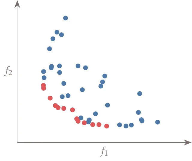
Figure 9.9:Population for a multiobjective GA iteration plotted against two objectives. The nondominated set is highlighted at the bottom left and eventually converges toward the Pareto front.

As the optimization progresses, the nondominated set moves further down and to the left and eventually converges toward the actual Pareto front.

In the multiobjective version of the GA, the reproduction and mutation phases are unchanged from the single-objective version. The primary difference is in determining the fitness and the selection procedure. Here, we provide an overview of one popular approach, the elitist nondominated sorting genetic algorithm (NSGA-II).^[2]

A step in the algorithm is to find a nondominated set (i.e., the current approximation of the Pareto set), and several algorithms exist to accomplish this. In the following, we use the algorithm by Kung et al.,9 which is one of the fastest. This procedure is described in Algorithm 9.1, where “front” is a shorthand for the nondominated set (which is just the current approximation of the Pareto front). The algorithm recursively divides the population in half and finds the nondominated set for each half separately.

Algorithm 9.1 (Find the nondominated set using Kung’s algorithm)

Algorithm

\quad ppp: A population sorted by the first objective
\quad fff: The nondominated set for the population
procedure front( ppp )
if length(ppp) = 1 then
If there is only one point, it is the frontSplit population into two halves ptp_tpt​ and pbp_bpb​
Because input was sorted, ptp_tpt​ will be superior to pbp_bpb​ in the first objective
ttt = front(ptp_tpt​) Recursive call to find front for top half
bbb = front(pbp_bpb​) Recursive call to find front for bottom half
Initialize fff with the members from ttt merged population
for i=1i = 1i=1 to  length(bbb) do
dominated = false Track whether anything in ttt dominates bib_ibi​
for j=1j = 1j=1 to  length(ttt) do
if tjt_jtj​ dominates bib_ibi​ then
dominated = true
break No need to continue search through ttt
if not dominated then
bib_ibi​ was not dominated by anything in tttAdd bib_ibi​ to fff
return  fff
end procedure

Before calling the algorithm, the population should be sorted by the first objective. First, we split the population into two halves, where the top half is superior to the bottom half in the first objective. Both populations are recursively fed back through the algorithm to find their nondominated sets. We then initialize a merged population with the members of the top half. All members in the bottom half are checked, and any that are nondominated by any member of the top half are added to the merged population. Finally, we return the merged population as the nondominated set.

With NSGA-II, in addition to determining the nondominated set, we want to rank all members by their dominance depth, which is also called nondominated sorting. In this approach, all nondominated points in the population (i.e., the current approximation of the Pareto set) are given a rank of 1. Those points are then removed from the set, and the next set of nondominated points is given a rank of 2, and so on.

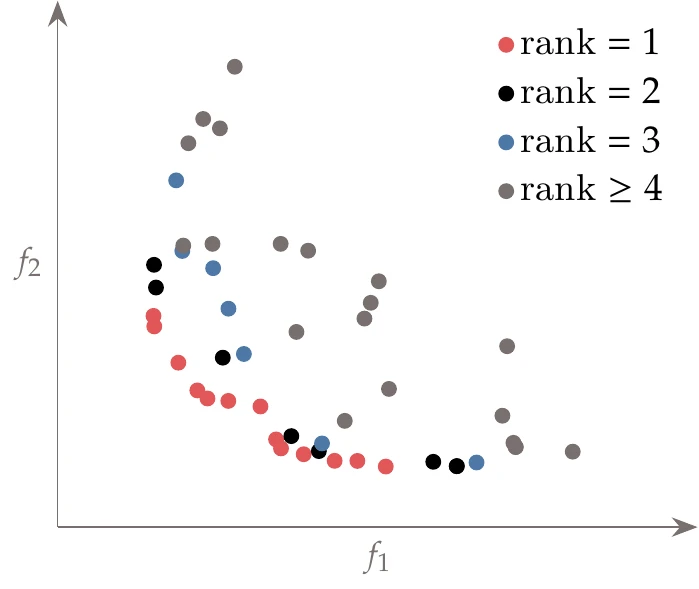
Figure 9.10:Points in the population highlighted by rank.

Figure 9.10 shows a sample population and illustrates the positions of the points with various rank values. There are alternative procedures that perform nondominated sorting directly, but we do not detail them here. This algorithm is summarized in Algorithm 9.2.

The new population in the GA is filled by placing all rank 1 points in the new population, then all rank 2 points, and so on. At some point, an entire group of constant rank will not fit within the new population. Points with the same rank are all equivalent as far as Pareto optimality is concerned, so an additional sorting mechanism is needed to determine which members of this group to include.

We perform selection within a group that can only partially fit to preserve diversity. Points in this last group are ordered by their crowding distance, which is a measure of how spread apart the points are. The algorithm seeks to preserve points that are well spread. For each point, a hypercube in objective space is formed around it, which, in NSGA-II, is referred to as a cuboid.

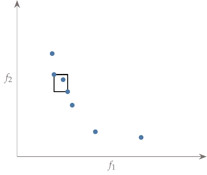
Figure 9.11:A cuboid around one point, demonstrating the definition of crowding distance (except that the distances are normalized).

Figure 9.11 shows an example cuboid considering the rank 3 points from Figure 9.10. The hypercube extends to the function values of its nearest neighbors in the function space. That does not mean that it necessarily touches its neighbors because the two closest neighbors can differ for each objective. The sum of the dimensions of this hypercube is the crowding distance.

When summing the dimensions, each dimension is normalized by the maximum range of that objective value. For example, considering only $f_1$ for the moment, if the objectives were in ascending order, then the contribution of point $i$ to the crowding distance would be

d_{1, i} = \frac{{f_1}_{i+1} - {f_1}_{i-1}}{{f_1}_{n_p} - {f_1}_{1}} \, .

(9.13)

where $n_p$ is the size of the population. Sometimes, instead of using the first and last points in the current objective set, user-supplied values are used for the min and max values of $f$ that appear in that denominator. The anchor points (the single-objective optima) are assigned a crowding distance of infinity because we want to preference their inclusion. The algorithm for crowding distance is shown in Algorithm 9.3.

We can now put together the overall multiobjective GA, as shown in Algorithm 9.4, where we use the components previously described (nondominated set, nondominated sorting, and crowding distance).

Algorithm 9.4 (Elitist nondominated sorting genetic algorithm)

Algorithm

\quad x‾\overline{x}x: Variable upper bounds
\quad x‾\underline{x}x​: Variable lower bounds
\quad x∗x^*x∗: Best point
Generate initial population
while Stopping criterion is not satisfied do
Using a parent population PPP, proceed as a standard GA for selection, crossover, and mutation, but use a crowded tournament selection to produced an offspring population OOO
C=P∪OC = P \cup OC=P∪O Combine populations
Compute ranki\text{rank}_iranki​ for i=1,2,…i = 1, 2, \ldotsi=1,2,… of CCC using Algorithm 9.2
Fill new parent population with as many whole ranks as possible
P=∅P = \emptysetP=∅
r=1r = 1r=1
while true do
set FFF as all CiC_iCi​ with ranki=r\text{rank}_i = rranki​=r
if length(PPP) + length(FFF) > npn_pnp​ then
add FFF to PPP
r=r+1r = r + 1r=r+1
For last rank that does not fit, add by crowding distance
if length(PPP)<np< n_p<np​ then
Population is not fulld = crowding(FFF) Algorithm 9.3, using last FFF from terminated previous loop
m=np−length(P)m = n_p - \text{length}(P)m=np​−length(P) Determine how many members to add
Sort FFF by the crowding distance ddd in descending order
Add the first mmm entries from FFF to PPP

The crossover and mutation operations remain the same. Tournament selection (Figure 7.25) is modified slightly to use this algorithm’s ranking and crowding metrics. In the tournament, a member with a lower rank is superior. If two members have the same rank, then the one with the larger crowding distance is selected. This procedure is called crowded tournament selection.

After reproduction and mutation, instead of replacing the parent generation with the offspring generation, both the parent generation and the offspring generation are saved as candidates for the next generation. This strategy is called elitism, which means that the best member in the population is guaranteed to survive.

The population size is now twice its original size ( $2n_p$ ), and the selection process must reduce the population back down to size $n_p$ . This is done using the procedure explained previously. The new population is filled by including all rank 1 members, rank 2 members, and so on until an entire rank can no longer fit. Inclusion for members of that last rank is done in the order of the largest crowding distance until the population is filled.

Many variations are possible, so although the algorithm is based on the concepts of NSGA-II, the details may differ somewhat.

The main advantage of this multiobjective approach is that if an evolutionary algorithm is appropriate for solving a given single-objective problem, then the extra information needed for a multiobjective problem is already there, and solving the multiobjective problem does not incur much additional computational cost. The pros and cons of this approach compared to the previous approaches are the same as those of gradient-based versus gradient-free methods, except that the multiobjective gradient-based approaches require solving multiple problems to generate the Pareto front. Still, solving multiple gradient-based problems may be more efficient than solving one gradient-free problem, especially for problems with a large number of design variables.

Example 9.4 (Filling a new population in NSGA-II)

After reproduction and mutation, we are left with a combined population of parents and offspring. In this small example, the combined population is of size 12, so we must reduce it back to 6. This example has two objectives, and the values for each member in the population are shown in the following table, where we assign a letter to each member. The population is plotted in Figure 9.12.

Figure 9.12:Population for this example.

	A	B	C	D	E	F	G	H	I	J	K	L
$f_1$	5	7	10	1	3	10	5	6	9	6	9	4
$f_2$	8	9	4	4	7	6	10	3	5	1	2	10

First, we compute the ranks using Algorithm 9.2, resulting in the following output:

A	B	C	D	E	F	G	H	I	J	K	L
3	4	3	1	2	4	4	2	3	1	2	3

We see that the current nondominated set consists of points D and J and that there are four different ranks.

Next, we start filling the new population in the order of rank. Our maximum capacity is 6, so all rank 1 {D, J} and rank 2 {E, H, K} fit. We cannot add rank 3 {A, C, I, L} because the population size would be 9. So far, our new population consists of {D, J, E, H, K}. To choose which items from rank 3 continue forward, we compute the crowding distance for the members of rank 3:

A	C	I	L
1.67	$\infty$	1.5	$\infty$

We would then add, in order {C, L, A, I}, but we only have room for one, so we add C and complete this iteration with a new population of {D, J, E, H, K, C}.

9.4 Summary¶

Multiobjective optimization is particularly useful in quantifying trade-off sensitivities between critical metrics. It is also useful when we seek a family of potential solutions rather than a single solution. Some scenarios where a family of solutions might be preferred include when the models used in optimization are low fidelity and higher-fidelity design tools will be applied or when more investigation is needed. A multiobjective approach can produce candidate solutions for later refinement.

The presence of multiple objectives changes what it means for a design to be optimal. A design is Pareto optimal when it is nondominated by any other design. The weighted-sum method is perhaps the most well-known approach, but it is not recommended because other methods are just as easy and much more efficient. The epsilon-constraint method is still simple yet almost always preferable to the weighted-sum method. It typically provides a better spaced Pareto front and can resolve any nonconvex portions of the front. If we are willing to use a more complex approach, the normal boundary intersection method is even more efficient at capturing a well-spaced Pareto front.

Some gradient-free methods, such as a multiobjective GA, can also generate Pareto fronts. If a gradient-free approach is a good fit in the single objective version of the problem, adding multiple objectives can be done with little extra cost. Although gradient-free methods are sometimes associated with multiobjective problems, gradient-based algorithms may be more effective for many multiobjective problems.

Problems¶

Exercise 1

Answer true or false and justify your answer.

The solution of multiobjective optimization problems is usually an infinite number of points.
It is advisable to include as many objectives as you can in your problem formulation to make sure you get the best possible design.
Multiobjective optimization can quantify trade-offs between objectives and constraints.
If the objectives are separable, that means that they can be minimized independently and that there is no Pareto front.
A point $A$ dominates point $B$ if it is better than $B$ in at least one objective.
The Pareto set is the set of points that dominate all other points in the objective space.
When a point is Pareto optimal, you cannot make either of the objectives better.
The weighted-sum method obtains the Pareto front by solving optimization problems with different objective functions.
The epsilon-constraint method obtains the Pareto front by constraining one objective and minimizing all the others.
The utopia point is the point where every objective has a minimum value.
It is not possible to compute a Pareto front with a single-objective optimizer.
Because GAs optimize by evolving a population of diverse designs, they can be used for multiobjective optimization without modification.

Footnotes¶

The first application of an evolutionary algorithm for solving a multiobjective problem was by 6
↩
The NSGA-II algorithm was developed by 7 Some key developments include using the concept of domination in the selection process, preserving diversity among the nondominated set, and using elitism.8
↩

References¶

Haimes, Y. Y., Lasdon, L. S., & Wismer, D. A. (1971). On a bicriterion formulation of the problems of integrated system identification and system optimization. IEEE Transactions on Systems, Man, and Cybernetics, SMC-1(3), 296–297. 10.1109/tsmc.1971.4308298
Das, I., & Dennis, J. E. (1998). Normal-boundary intersection: A new method for generating the Pareto surface in nonlinear multicriteria optimization problems. SIAM Journal on Optimization, 8(3), 631–657. 10.1137/s1052623496307510
Ismail-Yahaya, A., & Messac, A. (2002). Effective generation of the Pareto frontier using the normal constraint method. In Proceedings of the 40th AIAA Aerospace Sciences Meeting & Exhibit. American Institute of Aeronautics. 10.2514/6.2002-178
Messac, A., & Mattson, C. A. (2004). Normal constraint method with guarantee of even representation of complete Pareto frontier. AIAA Journal, 42(10), 2101–2111. 10.2514/1.8977
Hancock, B. J., & Mattson, C. A. (2013). The smart normal constraint method for directly generating a smart Pareto set. Structural and Multidisciplinary Optimization, 48(4), 763–775. 10.1007/s00158-013-0925-6
Schaffer, J. D. (1984). Some experiments in machine learning using vector evaluated genetic algorithms. [Phdthesis]. Vanderbilt University.
Deb, K., Pratap, A., Agarwal, S., & Meyarivan, T. (2002). A fast and elitist multiobjective genetic algorithm: NSGA-II. IEEE Transactions on Evolutionary Computation, 6(2), 182–197. 10.1109/4235.996017
Deb, K. (2008). Introduction to evolutionary multiobjective optimization. In Multiobjective Optimization (pp. 59–96). Springer. 10.1007/978-3-540-88908-3_3
Kung, H. T., Luccio, F., & Preparata, F. P. (1975). On finding the maxima of a set of vectors. Journal of the ACM, 22(4), 469–476. 10.1145/321906.321910

$f_1$	$f_2$
6.0	8.0
6.0	4.0
5.0	6.0
2.0	8.0
10.0	5.0
6.0	0.5
8.0	3.0
4.0	9.0
9.0	7.0
8.0	6.0
3.0	1.0
7.0	9.0
1.0	2.0
3.0	7.0
1.5	1.5
4.0	6.5