Appendix: Linear Solvers
In Section 3.6, we present an overview of solution methods for discretized systems of equations, followed by an introduction to Newton-based methods for solving nonlinear equations. Here, we review the solvers for linear systems required to solve for each step of Newton-based methods.[1]
B.1 Systems of Linear Equations
If the equations are linear, they can be written as
where is a square () matrix, and is a vector, and neither of these depends on . If this system of equations has a unique solution, then the system and the matrix are nonsingular. This is equivalent to saying that has an inverse, . If does not exist, the matrix and the system are singular.
A matrix is singular if its rows (or equivalently, its columns) are linearly dependent (i.e., if one of the rows can be written as a linear combination of the others).
If the matrix is nonsingular and we know its inverse , the solution of the linear system (Equation B.1) can be written as . However, the numerical methods described here do not form . The main reason for this is that forming is expensive: the computational cost is proportional to .
For practical problems with large , it is typical for the matrix to be sparse, that is, for most of its entries to be zeros. An entry represents the interaction between variables and . When solving differential equations on a discretized grid, for example, a given variable only interacts with variables in its vicinity in the grid. These interactions correspond to nonzero entries, whereas all other entries are zero. Sparse linear systems tend to have a number of nonzero terms that is proportional to . This is in contrast with a dense matrix, which has nonzero entries. Solvers should take advantage of sparsity to remain efficient for large .
We rewrite the linear system (Equation B.1) as a set of residuals,
To solve this system of equations, we can use either a direct method or an iterative method. We explain these briefly in the rest of this appendix, but we do not cover more advanced techniques that take advantage of sparsity.
B.2 Conditioning
The distinction between singular and nonsingular systems blurs once we have to deal with finite-precision arithmetic. Systems that are singular in the exact sense are ill-conditioned when a small change in the data (entries of or ) results in a large change in the solution. This large sensitivity of the solution to the problem parameters is an issue because the parameters themselves have finite precision. Then, any imprecision in these parameters can lead to significant errors in the solution, even if no errors are introduced in the numerical solution of the linear system.
The conditioning of a linear system can be quantified by the condition number of the matrix, which is defined as the scalar
where any matrix norm can be used.
Because , we have
for all matrices. A matrix is well-conditioned if is small and ill-conditioned if is large.
B.3 Direct Methods
The standard way to solve linear systems of equations with a computer is Gaussian elimination, which in matrix form is equivalent to LU factorization. This is a factorization (or decomposition) of , such as , where is a unit lower triangular matrix, and is an upper triangular matrix, as shown in Figure B.1.
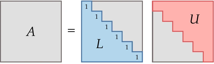
Figure B.1: factorization.
The factorization transforms the matrix into an upper triangular matrix by introducing zeros below the diagonal, one column at a time, starting with the first one and progressing from left to right. This is done by subtracting multiples of each row from subsequent rows. These operations can be expressed as a sequence of multiplications with lower triangular matrices ,
After completing these operations, we have , and we can find by computing .
Once we have this factorization, we have . Setting to , we can solve for by forward substitution. Now we have , which we can solve by back substitution for .
This process is not stable in general because roundoff errors are magnified in the backward substitution when diagonal elements of have a small magnitude. This issue is resolved by partial pivoting, which interchanges rows to obtain more favorable diagonal elements.
Cholesky factorization is an LU factorization specialized for the case where the matrix is symmetric and positive definite. In this case, pivoting is unnecessary because the Gaussian elimination is always stable for symmetric positive-definite matrices. The factorization can be written as
where .
This can be expressed as the matrix product
where .
B.4 Iterative Methods
Although direct methods are usually more efficient and robust, iterative methods have several advantages:
Iterative methods make it possible to trade between computational cost and precision because they can be stopped at any point and still yield an approximation of . On the other hand, direct methods only get the solution at the end of the process with the final precision.
Iterative methods have the advantage when a good guess for exists. This is often the case in optimization, where the from the previous optimization iteration can be used as the guess for the new evaluations (called a warm start).
Iterative methods do not require forming and manipulating the matrix , which can be computationally costly in terms of both time and memory. Instead, iterative methods require the computation of the residuals and, in the case of Krylov subspace methods, products of with a given vector. Therefore, iterative methods can be more efficient than direct methods for cases where is large and sparse. All that is needed is an efficient process to get the product of with a given vector, as shown in Figure B.2.
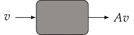
Figure B.2:Iterative methods just require a process (which can be a black box) to compute products of with an arbitrary vector .
Iterative methods are divided into stationary methods (also known as fixed-point iteration methods) and Krylov subspace methods.
B.4.1 Jacobi, Gauss–Seidel, and SOR
Fixed-point methods generate a sequence of iterates using a function
starting from an initial guess . The function is devised such that the iterates converge to the solution , which satisfies .
Many stationary methods can be derived by splitting the matrix such that . Then, leads to , and substituting this into the linear system yields
Because , substituting this into the previous equation results in the iteration
Defining the residual at iteration as
we can write
The splitting matrix is fixed and constructed so that it is easy to invert. The closer is to the inverse of , the better the iterations work.
We now introduce three stationary methods corresponding to three different splitting matrices.
The Jacobi method consists of setting to be a diagonal matrix , where the diagonal entries are those of . Then,
In component form, this can be written as
Using this method, each component in is independent of each other at a given iteration; they only depend on the previous iteration values, , and can therefore be done in parallel.
The Gauss–Seidel method is obtained by setting to be the lower triangular portion of and can be written as
where is the lower triangular matrix. Because of the triangular matrix structure, each component in is dependent on the previous elements in the vector, but the iteration can be performed in a single forward sweep. Writing this in component form yields
Unlike the Jacobi iterations, a Gauss–Seidel iteration cannot be performed in parallel because of the terms where , which require the latest values. Instead, the states must be updated sequentially. However, the advantage of Gauss–Seidel is that it generally converges faster than Jacobi iterations.
The successive over-relaxation (SOR) method uses an update that is a weighted average of the Gauss–Seidel update and the previous iteration,
where , the relaxation factor, is a scalar between 1 and 2. Setting yields the Gauss–Seidel method. SOR in component form is as follows:
With the correct value of , SOR converges faster than Gauss–Seidel.
B.4.2 Conjugate Gradient Method
The conjugate gradient method applies to linear systems where is symmetric and positive definite. This method can be adapted to solve nonlinear minimization problems (see Section 4.4.2).
We want to solve a linear system (Equation B.2) iteratively. This means that at a given iteration , the residual is not necessarily zero and can be written as
Solving this linear system is equivalent to minimizing the quadratic function
This is because the gradient of this function is
Thus, the gradient of the quadratic is the residual of the linear system,
We can express the path from any starting point to a solution as a sequence of steps with directions and length :
Substituting this into the quadratic (Equation B.20), we get
The conjugate gradient method uses a set of vectors that are conjugate with respect to matrix . Such vectors have the following property:
Using this conjugacy property, the double-sum term can be simplified to a single sum,
Then, Equation B.24 simplifies to
Because each term in this sum involves only one direction , we have reduced the original problem to a series of one-dimensional quadratic functions that can be minimized one at a time. Each one-dimensional problem corresponds to minimizing the quadratic with respect to the step length . Differentiating each term and setting it to zero yields the following:
Now, the question is: How do we find this set of directions? There are many sets of directions that satisfy conjugacy. For example, the eigenvectors of satisfy Equation B.25.[2]However, it is costly to compute the eigenvectors of a matrix. We want a more convenient way to compute a sequence of conjugate vectors.
The conjugate gradient method sets the first direction to the steepest-descent direction of the quadratic at the first point. Because the gradient of the function is the residual of the linear system (Equation B.22), this first direction is obtained from the residual at the starting point,
Each subsequent direction is set to a new conjugate direction using the update
where is set such that and are conjugate with respect to .
We can find the expression for by starting with the conjugacy property that we want to achieve,
Substituting the new direction with the update (Equation B.30), we get
Expanding the terms and solving for , we get
For each search direction , we can perform an exact line search by minimizing the quadratic analytically. The directional derivative of the quadratic at a point along the search direction is as follows:
By setting this derivative to zero, we can get the step size that minimizes the quadratic along the line to be
The numerator can be written as a function of the residual alone. Replacing with the conjugate direction update (Equation B.30), we get
Here we have used the property of the conjugate directions stating that the residual vector is orthogonal to all previous conjugate directions, so that for .[3] Thus, we can now write,
The numerator of the expression for (Equation B.33) can also be written in terms of the residual alone. Using the expression for the residual (Equation B.19) and taking the difference between two subsequent residuals, we get
Using this result in the numerator of in Equation B.33, we can write
where we have used the property that the residual at any conjugate residual iteration is orthogonal to the residuals at all previous iterations, so .[4]
Now, using this new numerator and using Equation B.37 to write the denominator as a function of the previous residual, we obtain
We use this result in the nonlinear conjugate gradient method for function minimization in Section 4.4.2.
The linear conjugate gradient steps are listed in Algorithm 2. The advantage of this method relative to the direct method is that does not need to be stored or given explicitly. Instead, we only need to provide a function that computes matrix-vector products with . These products are required to compute residuals () and the term in the computation of . Assuming a well-conditioned problem with good enough arithmetic precision, the algorithm should converge to the solution in steps.[5]
B.4.3 Krylov Subspace Methods
Krylov subspace methods are a more general class of iterative methods.[6] The conjugate gradient is a special case of a Krylov subspace method that applies only to symmetric positive-definite matrices. However, more general Krylov subspace methods, such as the generalized minimum residual (GMRES) method, do not have such restrictions on the matrix. Compared with stationary methods of Section B.4.1, Krylov methods have the advantage that they use information gathered throughout the iterations. Instead of using a fixed splitting matrix, Krylov methods effectively vary the splitting so that is changed at each iteration according to some criteria that use the information gathered so far. For this reason, Krylov methods are usually more efficient than stationary methods.
Like stationary iteration methods, Krylov methods do not require forming or storing . Instead, the iterations require only matrix-vector products of the form , where is some vector given by the Krylov algorithm. The matrix-vector product could be given by a black box, as shown in Figure B.2.
For the linear conjugate gradient method (Section B.4.2), we found conjugate directions and minimized the residual of the linear system in a sequence of these directions.
Krylov subspace methods minimize the residual in a space,
where is the initial guess, and is the Krylov subspace,
In other words, a Krylov subspace method seeks a solution that is a linear combination of the vectors . The definition of this particular sequence is convenient because these terms can be computed recursively with the matrix-vector product black box as .
Under certain conditions, it can be shown that the solution of the linear system of size is contained in the subspace .
Krylov subspace methods (including the conjugate gradient method) converge much faster when using preconditioning. Instead of solving , we solve
where is the preconditioning matrix (or simply preconditioner). The matrix should be similar to and correspond to a linear system that is easier to solve.
The inverse, , should be available explicitly, and we do not need an explicit form for . The matrix resulting from the product should have a smaller condition number so that the new linear system is better conditioned.
In the extreme case where , that means we have computed the inverse of , and we can get explicitly. In another extreme, could be a diagonal matrix with the diagonal elements of , which would scale such that the diagonal elements are 1.[7]Krylov subspace solvers require three main components: (1) an orthogonal basis for the Krylov subspace, (2) an optimal property that determines the solution within the subspace, and (3) an effective preconditioner. Various Krylov subspace methods are possible, depending on the choice for each of these three components. One of the most popular Krylov subspace methods is the GMRES.4[8]“‘
1 provides a much more detailed explanation of linear solvers.
Suppose we have two eigenvectors, and . Then . This dot product is zero because the eigenvectors of a symmetric matrix are mutually orthogonal.
Because the linear conjugate gradient method converges in steps, it was originally thought of as a direct method. It was initially dismissed in favor of more efficient direct methods, such as LU factorization. However, the conjugate gradient method was later reframed as an effective iterative method to obtain approximate solutions to large problems.
The splitting matrix we used in the equation for the stationary methods (Section B.4.1) is effectively a preconditioner. An using the diagonal entries of corresponds to the Jacobi method (Equation B.13).
GMRES and other Krylov subspace methods are available in most programming languages, including C/C++, Fortran, Julia, MATLAB, and Python.
- Trefethen, L. N., & Bau III, D. (1997). Numerical Linear Algebra. SIAM.
- Nocedal, J., & Wright, S. J. (2006). Numerical Optimization (2nd ed.). Springer. 10.1007/978-0-387-40065-5
- Saad, Y. (2003). Iterative Methods for Sparse Linear Systems (2nd ed.). SIAM. https://www.google.ca/books/edition/Iterative_Methods_for_Sparse_Linear_Syst/qtzmkzzqFmcC
- Saad, Y., & Schultz, M. H. (1986). GMRES: A generalized minimal residual algorithm for solving nonsymmetric linear systems. SIAM Journal on Scientific and Statistical Computing, 7(3), 856–869. 10.1137/0907058