Engineering design optimization problems are rarely unconstrained. In this chapter, we explain how to solve constrained problems. The methods in this chapter build on the gradient-based unconstrained methods from Chapter 4 and also assume smooth functions. We first introduce the optimality conditions for a constrained optimization problem and then focus on three main methods for handling constraints: penalty methods, sequential quadratic programming (SQP), and interior-point methods.
Penalty methods are no longer used in constrained gradient-based optimization because they have been replaced by more effective methods. Still, the concept of a penalty is useful when thinking about constraints, partially motivates more sophisticated approaches like interior-point methods, and is often used with gradient-free optimizers.
SQP and interior-point methods represent the state of the art in nonlinear constrained optimization. We introduce the basics for these two optimization methods, but a complete and robust implementation of these methods requires detailed knowledge of a growing body of literature that is not covered here.
where g(x) is the vector of inequality constraints, h(x) is the vector of equality constraints, and x and x are lower and upper design variable bounds (also known as bound constraints). Both objective and constraint functions can be nonlinear, but they should be C2 continuous to be solved using gradient-based optimization algorithms. The inequality constraints are expressed as “less than” without loss of generality because they can always be converted to “greater than” by putting a negative sign on g. We could also eliminate the equality constraints h=0 without loss of generality by replacing it with two inequality constraints, h≤ε and −h≤ε, where ε is some small number. In practice, it is desirable to distinguish between equality and inequality constraints because of numerical precision and algorithm implementation.
The constrained problem formulation just described does not distinguish between nonlinear and linear constraints. It is advantageous to make this distinction because some algorithms can take advantage of these differences. However, the methods introduced in this chapter assume general nonlinear functions.
For unconstrained gradient-based optimization (Chapter 4), we only require the gradient of the objective, ∇f. To solve a constrained problem, we also require the gradients of all the constraints. Because the constraints are vectors, their derivatives yield a Jacobian matrix. For the equality constraints, the Jacobian is defined as
which is an (nh×nx) matrix whose rows are the gradients of each constraint. Similarly, the Jacobian of the inequality constraints is an (ng×nx) matrix.
Understanding the optimality conditions and optimization algorithms for constrained problems requires basic n-dimensional geometry and linear algebra concepts. Here, we review the concepts in an informal way.[1] We sketch the concepts for two and three dimensions to provide some geometric intuition but keep in mind that the only way to tackle n dimensions is through mathematics.
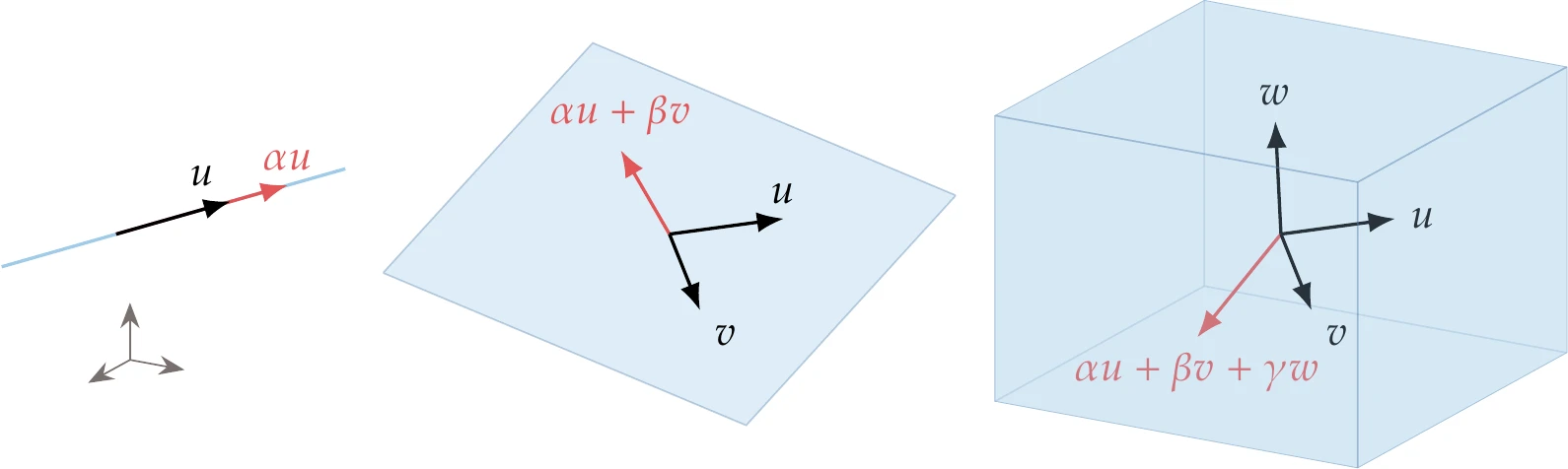
There are several essential linear algebra concepts for constrained optimization. The span of a set of vectors is the space formed by all the points that can be obtained by a linear combination of those vectors. With one vector, this space is a line, with two linearly independent vectors, this space is a two-dimensional plane (see Figure 5.2), and so on. With n linearly independent vectors, we can obtain any point in n-dimensional space.
Figure 5.2:Span of one, two, and three vectors in three-dimensional space.
Because matrices are composed of vectors, we can apply the concept of span to matrices. Suppose we have a rectangular (m×n) matrix A. For our purposes, we are interested in considering the m row vectors in the matrix.
The rank of A is the number of linearly independent rows of A, and it corresponds to the dimension of the space spanned by the row vectors of A.
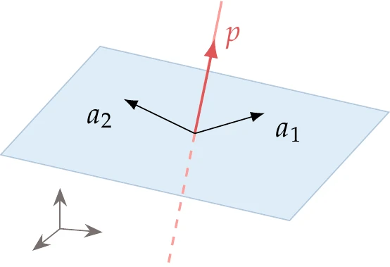
The nullspace of a matrix A is the set of all n-dimensional vectors p such that Ap=0.
Figure 5.3:Nullspace of a (2×3) matrix A of rank 2, where a1 and a2 are the row vectors of A.
This is a subspace of n−r dimensions, where r is the rank of A. One fundamental theorem of linear algebra is that the nullspace of a matrix contains all the vectors that are perpendicular to the row space of that matrix and vice versa. This concept is illustrated in Figure 5.3 for n=3, where r=2, leaving only one dimension for the nullspace. Any vector v that is perpendicular to p must be a linear combination of the rows of A, so it can be expressed as v=αa1+βa2.[2]A hyperplane is a generalization of a plane in n-dimensional space and is an essential concept in constrained optimization. In a space of n dimensions, a hyperplane is a subspace with at most n−1 dimensions. In Figure 5.4, we illustrate hyperplanes in two dimensions (a line) and three dimensions (a two-dimensional plane); higher dimensions cannot be visualized, but the mathematical description that follows holds for any n.
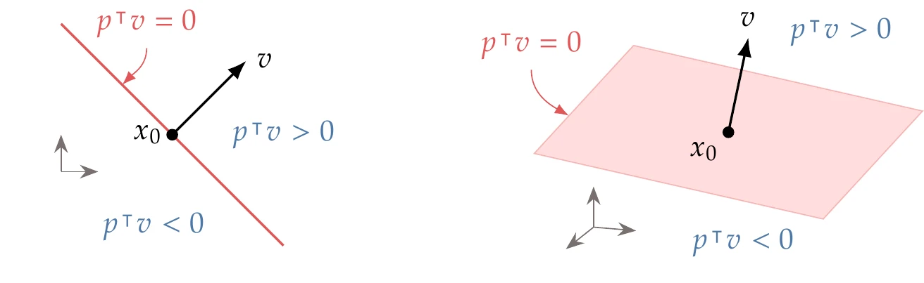
Figure 5.4:Hyperplanes and half-spaces in two and three dimensions.
To define a hyperplane of n−1 dimensions, we just need a point contained in the hyperplane (x0) and a vector (v). Then, the hyperplane is defined as the set of all points x=x0+p such that p⊺v=0. That is, the hyperplane is defined by all vectors that are perpendicular to v. To define a hyperplane with n−2 dimensions, we would need two vectors, and so on. In n dimensions, a hyperplane of n−1 dimensions divides the space into two half-spaces: in one of these, p⊺v>0, and in the other, p⊺v<0. Each half-space is closed if it includes the hyperplane (p⊺v=0) and open otherwise.
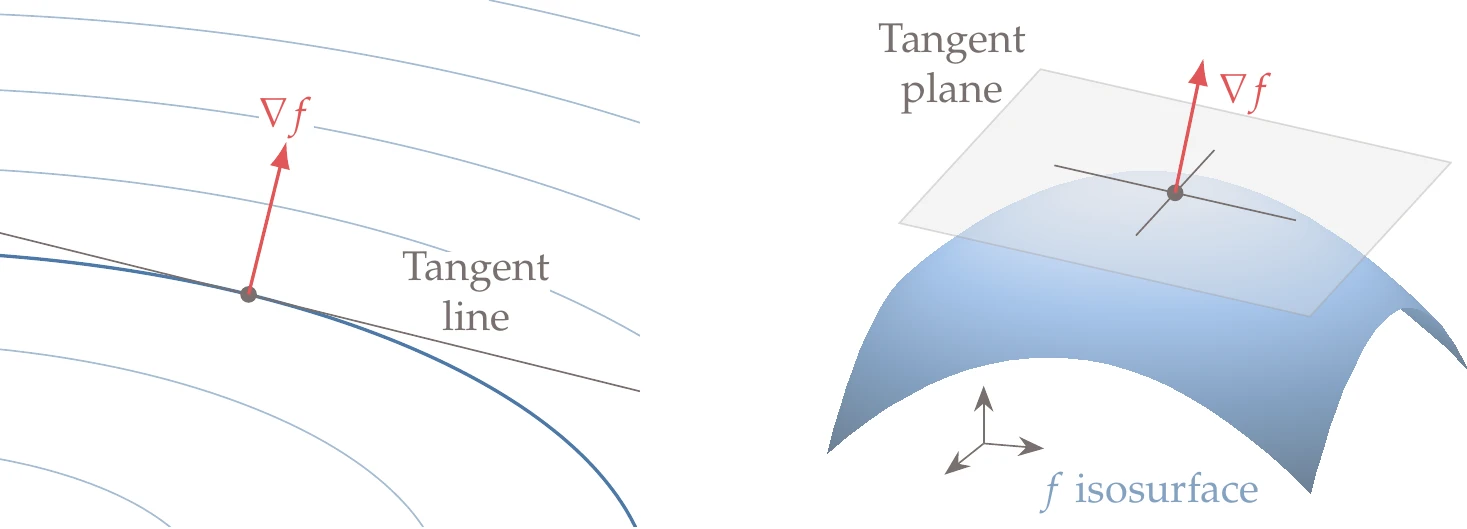
When we have the isosurface of a function f, the function gradient at a point on the isosurface is locally perpendicular to the isosurface. The gradient vector defines the tangent hyperplane at that point, which is the set of points such that p⊺∇f=0. In two dimensions, the isosurface reduces to a contour and the tangent reduces to a line, as shown in Figure 5.5 (left). In three dimensions, we have a two-dimensional hyperplane tangent to an isosurface, as shown in Figure 5.5 (right).
Figure 5.5:The gradient of a function defines the hyperplane tangent to the function isosurface.
The intersection of multiple half-spaces yields a polyhedral cone.
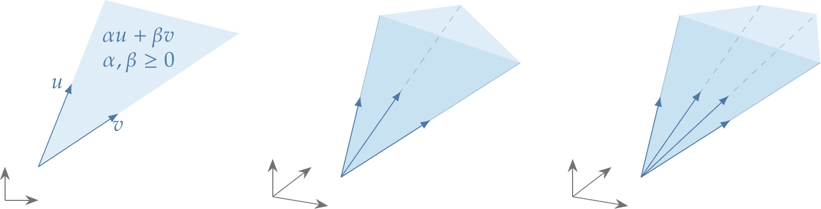
A polyhedral cone is the set of all the points that can be obtained by the linear combination of a given set of vectors using nonnegative coefficients. This concept is illustrated in Figure 5.6 (left) for the two-dimensional case.
In this case, only two vectors are required to define a cone uniquely. In three dimensions and higher there could be any number of vectors corresponding to all the possible polyhedral “cross sections”, as illustrated in Figure 5.6 (middle and right).
Figure 5.6:Polyhedral cones in two and three dimensions.
The optimality conditions for constrained optimization problems are not as straightforward as those for unconstrained optimization (Section 4.1.4). We begin with equality constraints because the mathematics and intuition are simpler, then add inequality constraints. As in the case of unconstrained optimization, the optimality conditions for constrained problems are used not only for the termination criteria, but they are also used as the basis for optimization algorithms.
First, we review the optimality conditions for an unconstrained problem, which we derived in Section 4.1.4. For the unconstrained case, we can take a first-order Taylor series expansion of the objective function with some step p that is small enough that the second-order term is negligible and write
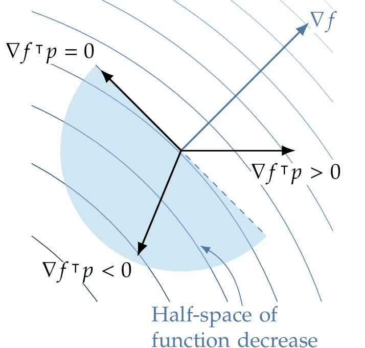
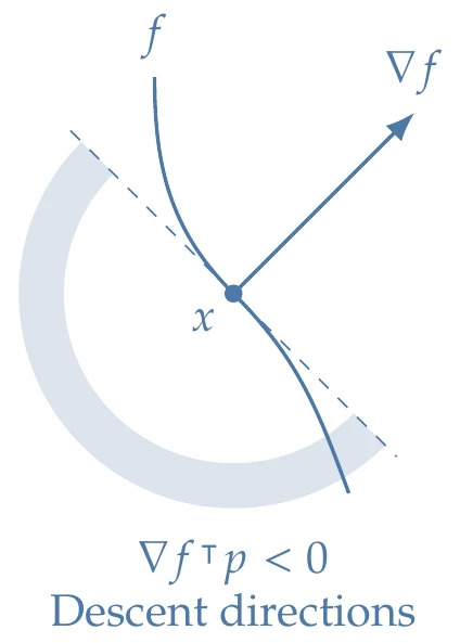
The condition ∇f⊺p=0 defines a hyperplane that contains the directions along which the first-order variation of the function is zero. This hyperplane divides the space into an open half-space of directions where the function decreases (∇f⊺p<0) and an open half-space where the function increases (∇f⊺p>0), as shown in Figure 5.7. Again, we are considering first-order variations.
Figure 5.7:The gradient f(x), which is the direction of steepest function increase, splits the design space into two halves. Here we highlight the open half-space of directions that result in function decrease.
If the problem were unconstrained, the only way to satisfy the inequality in Equation 5.5 would be if ∇f(x∗)=0. That is because for any nonzero ∇f, there is an open half-space of directions that result in a function decrease (see Figure 5.7). This is consistent with the first-order unconstrained optimality conditions derived in Section 4.1.4.
However, we now have a constrained problem. The function increase condition (Equation 5.5) still applies, but p must also be a feasible direction. To find the feasible directions, we can write a first-order Taylor series expansion for each equality constraint function as
Again, the step size is assumed to be small enough so that the higher-order terms are negligible.
Assuming that x is a feasible point, then hj(x)=0 for all constraints j, and we are left with the second term in the linearized constraint (Equation 5.6). To remain feasible a small step away from x, we require that hj(x+p)=0 for all j. Therefore, first-order feasibility requires that
This equation states that any feasible direction has to lie in the nullspace of the Jacobian of the constraints, Jh.
Figure 5.8:If we have two equality constraints (nh=2) in two-dimensional space (nx=2), we are left with no freedom for optimization.
Assuming that Jh has full row rank (i.e., the constraint gradients are linearly independent), then the feasible space is a subspace of dimension nx−nh. For optimization to be possible, we require nx>nh. Figure 5.8 illustrates a case where nx=nh=2, where the feasible space reduces to a single point, and there is no freedom for performing optimization.
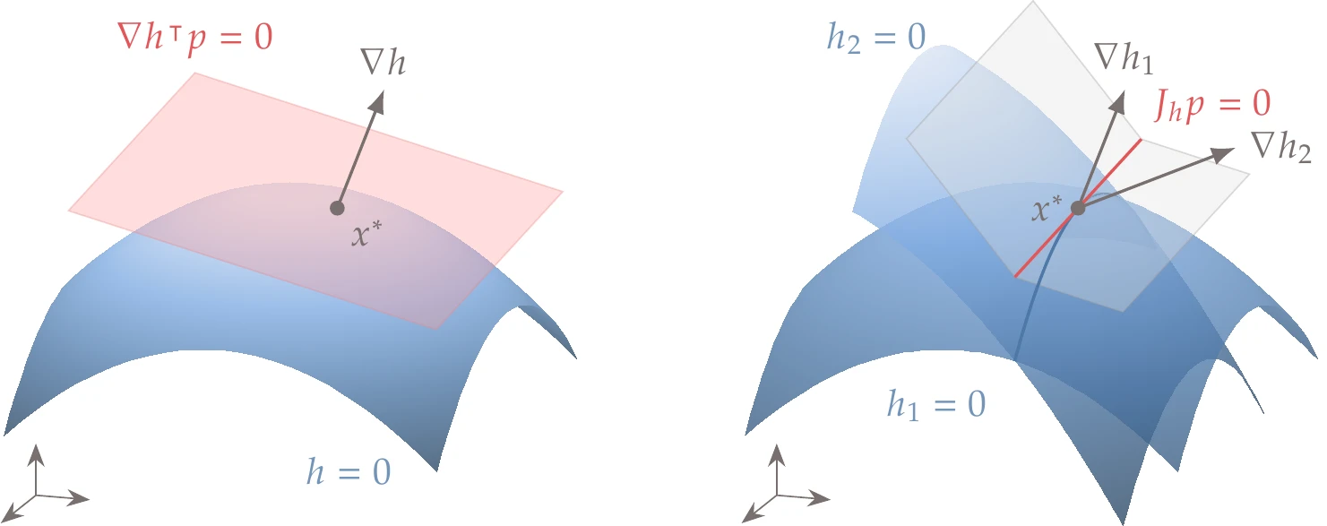
For one constraint, Equation 5.8 reduces to a dot product, and the feasible space corresponds to a tangent hyperplane, as illustrated on the left side of Figure 5.9 for the three-dimensional case. For two or more constraints, the feasible space corresponds to the intersection of all the tangent hyperplanes. On the right side of Figure 5.9, we show the intersection of two tangent hyperplanes in three-dimensional space (a line).
Figure 5.9:Feasible spaces in three dimensions for one and two constraints.
For constrained optimality, we need to satisfy both ∇f(x∗)⊺p≥0 (Equation 5.5) and Jh(x)p=0 (Equation 5.8). For equality constraints, if a direction p is feasible, then −p must also be feasible. Therefore, the only way to satisfy ∇f(x∗)⊺p≥0 is if ∇f(x)⊺p=0.
In sum, for x∗ to be a constrained optimum, we require
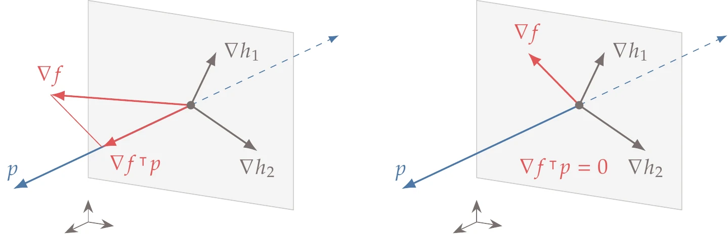
In other words, the projection of the objective function gradient onto the feasible space must vanish. Figure 5.10 illustrates this requirement for a case with two constraints in three dimensions.
Figure 5.10:If the projection of ∇f onto the feasible space is nonzero, there is a feasible descent direction (left); if the projection is zero, the point is a constrained optimum (right).
The constrained optimum conditions (Equation 5.9) require that ∇f be orthogonal to the nullspace of Jh (since p, as defined, is the nullspace of Jh). The row space of a matrix contains all the vectors that are orthogonal to its nullspace.[3]Because the rows of Jh are the gradients of the constraints, the objective function gradient must be a linear combination of the gradients of the constraints. Thus, we can write the requirements defined in Equation 5.9 as a single vector equation,
where λj are called the Lagrange multipliers.[4]There is a multiplier associated with each constraint. The sign of the Lagrange multipliers is arbitrary for equality constraints but will be significant later when dealing with inequality constraints.
Therefore, the first-order optimality conditions for the equality constrained case are
In this function, the Lagrange multipliers are considered to be independent variables. Taking the gradient of L with respect to both x and λ and setting them to zero yields
which are the first-order conditions derived in Equation 5.11.
With the Lagrangian function, we have transformed a constrained problem into an unconstrained problem by adding new variables, λ. A constrained problem of nx design variables and nh equality constraints was transformed into an unconstrained problem with nx+nh variables. Although you might be tempted to simply use the algorithms of Chapter 4 to minimize the Lagrangian function (Equation 5.12), some modifications are needed in the algorithms to solve these problems effectively (particularly once inequality constraints are introduced).
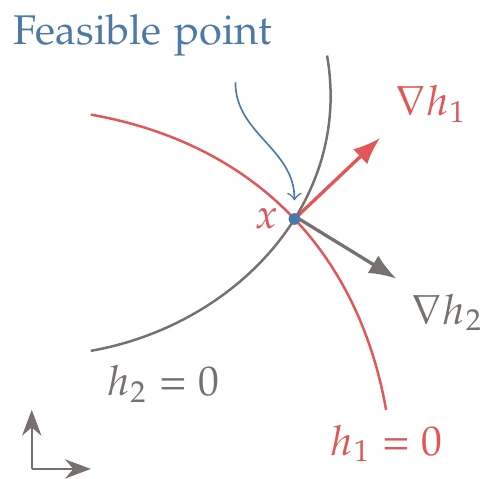
Figure 5.11:The constraint qualification condition does not hold in this case because the gradients of the two constraints not linearly independent.
The derivation of the first-order optimality conditions (Equation 5.11) assumes that the gradients of the constraints are linearly independent; that is, Jh has full row rank. A point satisfying this condition is called a regular point and is said to satisfy linear independence constraint qualification. Figure 5.11 illustrates a case where the x∗ is not a regular point. A special case that does not satisfy constraint qualification is when one (or more) constraint gradient is zero. In that case, that constraint is not linearly independent, and the point is not regular. Fortunately, these situations are uncommon.
The optimality conditions just described are first-order conditions that are necessary but not sufficient. To make sure that a point is a constrained minimum, we also need to satisfy second-order conditions. For the unconstrained case, the Hessian of the objective function has to be positive definite. In the constrained case, we need to check the Hessian of the Lagrangian with respect to the design variables in the space of feasible directions. The Lagrangian Hessian is
We can reuse some of the concepts from the equality constrained optimality conditions for inequality constrained problems.
Recall that an inequality constraint j is feasible when gj(x∗)≤0 and it is said to be active if gj(x∗)=0 and inactive if gj(x∗)<0.
Figure 5.15:The descent directions are in the open half-space defined by the objective function gradient.
As before, if x∗ is an optimum, any small enough feasible step p from the optimum must result in a function increase. Based on the Taylor series expansion (Equation 5.3), we get the condition
which is the same as for the equality constrained case. We use the arc in Figure 5.15 to show the descent directions, which are in the open half-space defined by the hyperplane tangent to the gradient of the objective.
To consider inequality constraints, we use the same linearization as the equality constraints (Equation 5.6), but now we enforce an inequality to get
For a given candidate point that satisfies all constraints, there are two possibilities to consider for each inequality constraint: whether the constraint is inactive (gj(x)<0) or active (gj(x)=0). If a given constraint is inactive, we do not need to add any condition for it because we can take a step p in any direction and remain feasible as long as the step is small enough. Thus, we only need to consider the active constraints for the optimality conditions.
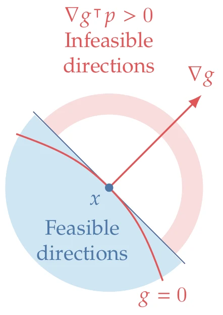
Figure 5.16:The feasible directions for each constraint are in the closed half-space defined by the inequality constraint gradient.
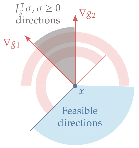
For the equality constraint, we found that all first-order feasible directions are in the nullspace of the Jacobian matrix. Inequality constraints are not as restrictive. From Equation 5.17, if constraint j is active (gj(x)=0), then the nearby point gj(x+p) is only feasible if ∇gj(x)⊺p≤0 for all constraints j that are active. In matrix form, we can write Jg(x)p≤0, where the Jacobian matrix includes only the gradients of the active constraints. Thus, the feasible directions for inequality constraint j can be any direction in the closed half-space, corresponding to all directions p such that p⊺gj≤0, as shown in Figure 5.16. In this figure, the arc shows the infeasible directions.
The set of feasible directions that satisfies all active constraints is the intersection of all the closed half-spaces defined by the inequality constraints, that is, all p such that Jg(x)p≤0. This intersection of the feasible directions forms a polyhedral cone, as illustrated in Figure 5.17 for a two-dimensional case with two constraints.
Figure 5.17:Excluding the infeasible directions with respect to each constraint (red arcs) leaves the cone of feasible directions (blue), which is the polar cone of the active constraint gradients cone (gray).
To find the cone of feasible directions, let us first consider the cone formed by the active inequality constraint gradients (shown in gray in Figure 5.17). This cone is defined by all vectors d such that
A direction p is feasible if p⊺d≤0 for all d in the cone. The set of all feasible directions forms the polar cone of the cone defined by Equation 5.18 and is shown in blue in Figure 5.17.
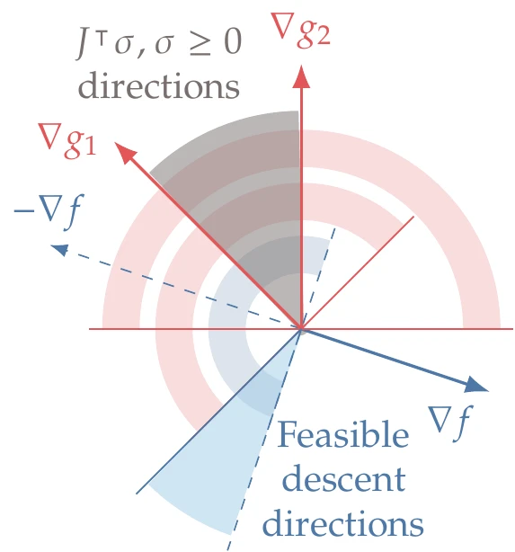
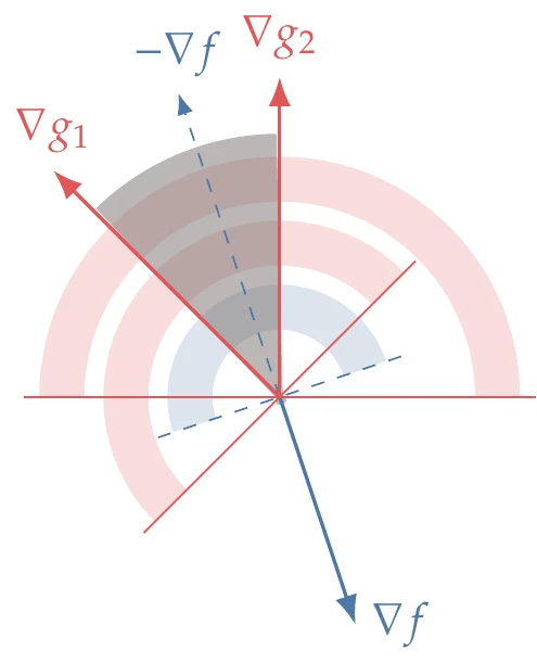
Now that we have established some intuition about the feasible directions, we need to establish under which conditions there is no feasible descent direction (i.e., we have reached an optimum). In other words, when is there no intersection between the cone of feasible directions and the open half-space of descent directions? To answer this question, we can use Farkas’ lemma. This lemma states that given a rectangular matrix (Jg in our case) and a vector with the same size as the rows of the matrix (∇f in our case), one (and only one) of two possibilities occurs:[7]
There exists a p such that Jgp≤0 and ∇f⊺p<0. This means that there is a descent direction that is feasible (Figure 5.18, left).
There exists a σ such that Jg⊺σ=−∇f with σ≥0 (Figure 5.18, right). This corresponds to optimality because it excludes the first possibility.
Comparing with the corresponding criteria for equality constraints (Equation 5.13), we see a similar form. However, σ corresponds to the Lagrange multipliers for the inequality constraints and carries the additional restriction that σ≥0.
If equality constraints are present, the conditions for the inequality constraints apply only in the subspace of the directions feasible with respect to the equality constraints.
Similar to the equality constrained case, we can construct a Lagrangian function whose stationary points are candidates for optimal points. We need to include all inequality constraints in the optimality conditions because we do not know in advance which constraints are active. To represent inequality constraints in the Lagrangian, we replace them with the equality constraints defined by
where sj is a new unknown associated with each inequality constraint called a slack variable. The slack variable is squared to ensure it is nonnegative In that way, Equation 5.20 can only be satisfied when gj is feasible (gj≤0).
The significance of the slack variable is that when sj=0, the corresponding inequality constraint is active (gj=0), and when sj=0, the corresponding constraint is inactive.
The Lagrangian including both equality and inequality constraints is then
where σ represents the Lagrange multipliers associated with the inequality constraints. Here, we use ⊙ to represent the element-wise multiplication of s.[8]Similar to the equality constrained case, we seek a stationary point for the Lagrangian, but now we have additional unknowns: the inequality Lagrange multipliers and the slack variables. Taking partial derivatives of the Lagrangian with respect to each set of unknowns and setting those derivatives to zero yields the first-order optimality conditions:
This criterion is the same as before but with additional Lagrange multipliers and constraints. Taking the derivatives with respect to the equality Lagrange multipliers, we have
which is called the complementary slackness condition. This condition helps us to distinguish the active constraints from the inactive ones. For each inequality constraint, either the Lagrange multiplier is zero (which means that the constraint is inactive), or the slack variable is zero (which means that the constraint is active). Unfortunately, the complementary slackness condition introduces a combinatorial problem. The complexity of this problem grows exponentially with the number of inequality constraints because the number of possible combinations of active versus inactive constraints is 2ng.
In addition to the conditions for a stationary point of the Lagrangian (Equation 5.22, Equation 5.23, Equation 5.24, and Equation 5.25), recall that we require the Lagrange multipliers for the active constraints to be nonnegative. Putting all these conditions together in matrix form, the first-order constrained optimality conditions are as follows:
These are called the Karush–Kuhn–Tucker (KKT) conditions. The equality and inequality constraints are sometimes lumped together using a single Jacobian matrix (and single Lagrange multiplier vector). This can be convenient because the expression for the Lagrangian follows the same form for both cases.
As in the equality constrained case, these first-order conditions are necessary but not sufficient. The second-order sufficient conditions require that the Hessian of the Lagrangian must be positive definite in all feasible directions, that is,
p⊺HLpJhpJgp>0for all p such that:=0≤0for the active constraints.
In other words, we only require positive definiteness in the intersection of the nullspace of the equality constraint Jacobian with the feasibility cone of the active inequality constraints.
Similar to the equality constrained case, the KKT conditions (Equation 5.26) only apply when a point is regular, that is, when it satisfies linear independence constraint qualification. However, the linear independence applies only to the gradients of the inequality constraints that are active and the equality constraint gradients.
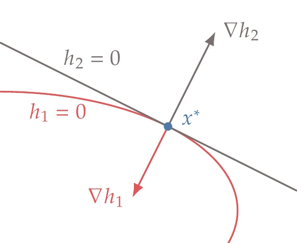
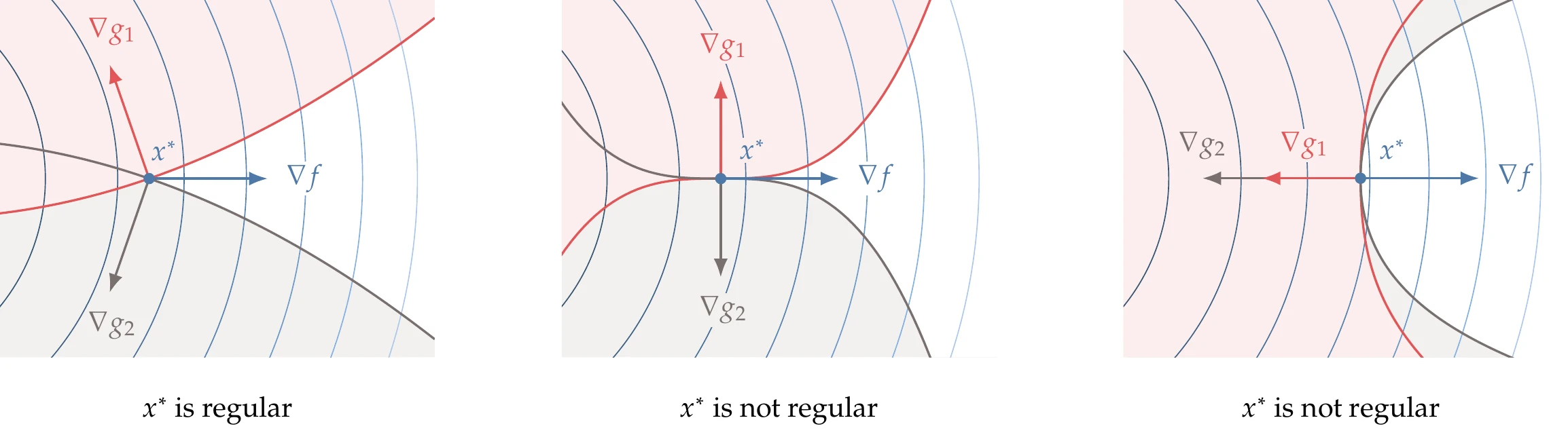
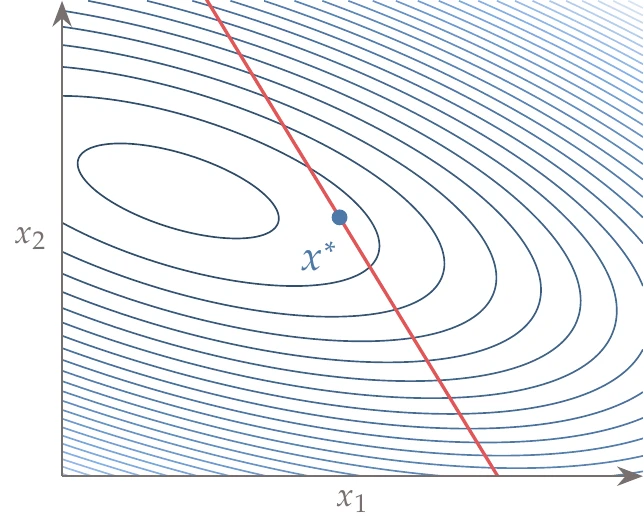
Suppose we have the two constraints shown in the left pane of Figure 5.19. For the given objective function contours, point x∗ is a minimum. At x∗, the gradients of the two constraints are linearly independent, and x∗ is thus a regular point. Therefore, we can apply the KKT conditions at this point.
Figure 5.19:The KKT conditions apply only to regular points. A point x∗ is regular when the gradients of the constraints are linearly independent. The middle and right panes illustrate cases where x∗ is a constrained minimum but not a regular point.
The middle and right panes of Figure 5.19 illustrate cases where x∗ is also a constrained minimum. However, x∗ is not a regular point in either case because the gradients of the two constraints are not linearly independent. This means that the gradient of the objective cannot be expressed as a unique linear combination of the constraints. Therefore, we cannot use the KKT conditions, even though x∗ is a minimum. The problem would be ill-conditioned, and the numerical methods described in this chapter would run into numerical difficulties. Similar to the equality constrained case, this situation is uncommon in practice.
Although these examples can be solved analytically, they are the exception rather than the rule. The KKT conditions quickly become challenging to solve analytically (try solving Example 5.1), and as the number of constraints increases, trying all combinations of active and inactive constraints becomes intractable. Furthermore, engineering problems usually involve functions defined by models with implicit equations, which are impossible to solve analytically. The reason we include these analytic examples is to gain a better understanding of the KKT conditions. For the rest of the chapter, we focus on numerical methods, which are necessary for the vast majority of practical problems.
The Lagrange multipliers quantify how much the corresponding constraints drive the design. More specifically, a Lagrange multiplier quantifies the sensitivity of the optimal objective function value f(x∗) to a variation in the value of the corresponding constraint. Here we explain why that is the case. We discuss only inequality constraints, but the same analysis applies to equality constraints.
When a constraint is inactive, the corresponding Lagrange multiplier is zero. This indicates that changing the value of an inactive constraint does not affect the optimum, as expected. This is only valid to the first order because the KKT conditions are based on the linearization of the objective and constraint functions. Because small changes are assumed in the linearization, we do not consider the case where an inactive constraint becomes active after perturbation.
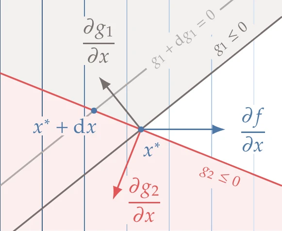
Now let us examine the active constraints. Suppose that we want to quantify the effect of a change in an active (or equality) constraint gi on the optimal objective function value.[9]The differential of gi is given by the following dot product:
This equation states that any movement dx must be in the nullspace of the remaining constraints to remain feasible with respect to those constraints.[10]An example with two constraints is illustrated in Figure 5.24, where g1 is perturbed and g2 remains fixed. The objective and constraint functions are linearized because we are considering first-order changes represented by the differentials.
Figure 5.24:Lagrange multipliers can be interpreted as the change in the optimal objective due a perturbation in the corresponding constraint. In this case, we show the effect of perturbing g1.
From the KKT conditions (Equation 5.22), we know that at the optimum,
Thus, the Lagrange multipliers can predict how much improvement can be expected if a given constraint is relaxed. For inequality constraints, because the Lagrange multipliers are positive at an optimum, this equation correctly predicts a decrease in the objective function value when the constraint value is increased.
The derivative defined in Equation 5.33 has practical value because it tells us how much a given constraint drives the design. In this interpretation of the Lagrange multipliers, we need to consider the scaling of the problem and the units. Still, for similar quantities, they quantify the relative importance of the constraints.
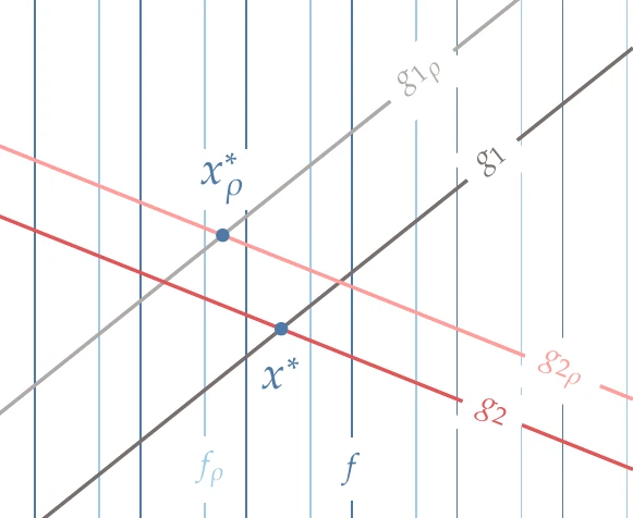
It is sometimes helpful to find sensitivities of the optimal objective function value with respect to a parameter held fixed during optimization. Suppose that we have found the optimum for a constrained problem. Say we have a scalar parameter ρ held fixed in the optimization, but now want to quantify the effect of a perturbation in that parameter on the optimal objective value. Perturbing ρ changes the objective and the constraint functions, so the optimum point moves, as illustrated in Figure 5.25. For our current purposes, we use g to represent either active inequality or equality constraints.
We assume that the set of active constraints does not change with a perturbation in ρ like we did when perturbing the constraint in Section 5.3.3.
Figure 5.25:Post-optimality sensitivities quantify the change in the optimal objective due to a perturbation of a parameter that was originally fixed in the optimization.
The optimal objective value changes due to changes in the optimum point (which moves to xρ∗) and objective function (which becomes fρ.)
The objective function is affected by ρ through a change in f itself and a change induced by the movement of the constraints. This dependence can be written in the total differential form as:
The derivative ∂f/∂g corresponds to the derivative of the optimal value of the objective with respect to a perturbation in the constraint, which according to Equation 5.33, is the negative of the Lagrange multipliers. This means that the post-optimality derivative is
The concept behind penalty methods is intuitive: to transform a constrained problem into an unconstrained one by adding a penalty to the objective function when constraints are violated or close to being violated. As mentioned in the introduction to this chapter, penalty methods are no longer used directly in gradient-based optimization algorithms because they have difficulty converging to the true solution. However, these methods are still valuable because (1) they are simple and thus ease the transition into understanding constrained optimization; (2) they are useful in some constrained gradient-free methods (Chapter 7); (3) they can be used as merit functions in line search algorithms, as discussed in Section 5.5.3; (4) penalty concepts are used in interior points methods, as discussed in Section 5.6.
where π(x) is a penalty function, and the scalar μ is a penalty parameter. This is similar in form to the Lagrangian, but one difference is that μ is fixed instead of being a variable.
We can use the unconstrained optimization techniques to minimize f^(x). However, instead of just solving a single optimization problem, penalty methods usually solve a sequence of problems with different values of μ to get closer to the actual constrained minimum. We will see shortly why we need to solve a sequence of problems rather than just one problem.
Various forms for π(x) can be used, leading to different penalty methods. There are two main types of penalty functions: exterior penalties, which impose a penalty only when constraints are violated, and interior penalty functions, which impose a penalty that increases as a constraint is approached.
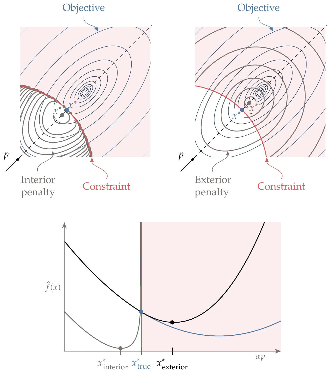
Figure 5.26 shows both interior and exterior penalties for a two-dimensional function. The exterior penalty leads to slightly infeasible solutions, whereas an interior penalty leads to a feasible solution but underpredicts the objective.
Figure 5.26:Interior penalties tend to infinity as the constraint is approached from the feasible side of the constraint (left), whereas exterior penalty functions activate when the points are not feasible (right). The minimum for both approaches is different from the true constrained minimum.
Of the many possible exterior penalty methods, we focus on two of the most popular ones: quadratic penalties and the augmented Lagrangian method. Quadratic penalties are continuously differentiable and straightforward to implement, but they suffer from numerical ill-conditioning. The augmented Lagrangian method is more sophisticated; it is based on the quadratic penalty but adds terms that improve the numerical properties. Many other penalties are possible, such as 1-norms, which are often used when continuous differentiability is unnecessary.
where the semicolon denotes that μ is a fixed parameter. The motivation for a quadratic penalty is that it is simple and results in a function that is continuously differentiable. The factor of one half is unnecessary but is included by convention because it eliminates the extra factor of two when taking derivatives. The penalty is nonzero unless the constraints are satisfied (hi=0), as desired.
Figure 5.27:Quadratic penalty for an equality constrained problem. The minimum of the penalized function (black dots) approaches the true constrained minimum (blue circle) as the penalty parameter μ increases.
The value of the penalty parameter μ must be chosen carefully. Mathematically, we recover the exact solution to the constrained problem only as μ tends to infinity (see Figure 5.27). However, starting with a large value for μ is not practical. This is because the larger the value of μ, the larger the Hessian condition number, which corresponds to the curvature varying greatly with direction (see Example 4.10). This behavior makes the problem difficult to solve numerically.
To solve the problem more effectively, we begin with a small value of μ and solve the unconstrained problem. We then increase μ and solve the new unconstrained problem, using the previous solution as the starting point. We repeat this process until the optimality conditions (or some other approximate convergence criteria) are satisfied, as outlined in Algorithm 5.1. By gradually increasing μ and reusing the solution from the previous problem, we avoid some of the ill-conditioning issues. Thus, the original constrained problem is transformed into a sequence of unconstrained optimization problems.
There are three potential issues with the approach outlined in Algorithm 5.1. Suppose the starting value for μ is too low. In that case, the penalty might not be enough to overcome a function that is unbounded from below, and the penalized function has no minimum.
The second issue is that we cannot practically approach μ→∞. Hence, the solution to the problem is always slightly infeasible. By comparing the optimality condition of the constrained problem,
Because hj=0 at the optimum, μ must be large to satisfy the constraints.
The third issue has to do with the curvature of the penalized function, which is directly proportional to μ. The extra curvature is added in a direction perpendicular to the constraints, making the Hessian of the penalized function increasingly ill-conditioned as μ increases. Thus, the need to increase μ to improve accuracy directly leads to a function space that is increasingly challenging to solve.
The approach discussed so far handles only equality constraints, but we can extend it to handle inequality constraints. Instead of adding a penalty to both sides of the constraints, we add the penalty when the inequality constraint is violated (i.e., when gj(x)>0). This behavior can be achieved by defining a new penalty function as
The only difference relative to the equality constraint penalty shown in Figure 5.27 is that the penalty is removed on the feasible side of the inequality constraint, as shown in Figure 5.30.
Figure 5.30:Quadratic penalty for an inequality constrained problem. The minimum of the penalized function approaches the constrained minimum from the infeasible side.
The inequality quadratic penalty can be used together with the quadratic penalty for equality constraints if we need to handle both types of constraints:
As explained previously, the quadratic penalty method requires a large value of μ for constraint satisfaction, but the large μ degrades the numerical conditioning. The augmented Lagrangian method helps alleviate this dilemma by adding the quadratic penalty to the Lagrangian instead of just adding it to the function. The augmented Lagrangian function for equality constraints is
This approach is an improvement on the plain quadratic penalty because updating the Lagrange multiplier estimates at each iteration allows for more accurate solutions without increasing μ as much. The augmented Lagrangian approximation for each constraint obtained from Equation 5.49 is
The quadratic penalty relies solely on increasing μ in the denominator to drive the constraints to zero.
However, the augmented Lagrangian also controls the numerator through the Lagrange multiplier estimate. If the estimate is reasonably close to the true Lagrange multiplier, then the numerator becomes small for modest values of μ. Thus, the augmented Lagrangian can provide a good solution for x∗ while avoiding the ill-conditioning issues of the quadratic penalty.
So far we have only discussed equality constraints where the definition for the augmented Lagrangian is universal. Example 5.8 included an inequality constraint by assuming it was active and treating it like an equality, but this is not an approach that can be used in general. Several formulations exist for handling inequality constraints using the augmented Lagrangian approach.456 One well-known approach is given by:7
Interior penalty methods work the same way as exterior penalty methods—they transform the constrained problem into a series of unconstrained problems. The main difference with interior penalty methods is that they always seek to maintain feasibility. Instead of adding a penalty only when constraints are violated, they add a penalty as the constraint is approached from the feasible region. This type of penalty is particularly desirable if the objective function is ill-defined outside the feasible region. These methods are called interior because the iteration points remain on the interior of the feasible region. They are also referred to as barrier methods because the penalty function acts as a barrier preventing iterates from leaving the feasible region.
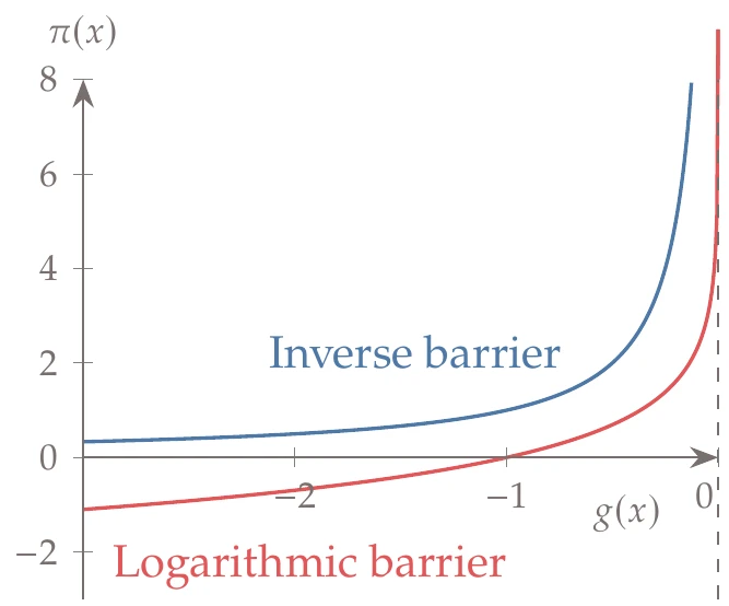
Figure 5.34:Two different interior penalty functions: inverse barrier and logarithmic barrier.
One possible interior penalty function to enforce g(x)≤0 is the inverse barrier,
where π(x)→∞ as gj(x)→0− (where the superscript “−” indicates a left-sided derivative). A more popular interior penalty function is the logarithmic barrier,
These two penalty functions as illustrated in Figure 5.34.
Neither of these penalty functions applies when g>0 because they are designed to be evaluated only within the feasible space. Algorithms based on these penalties must be prevented from evaluating infeasible points.
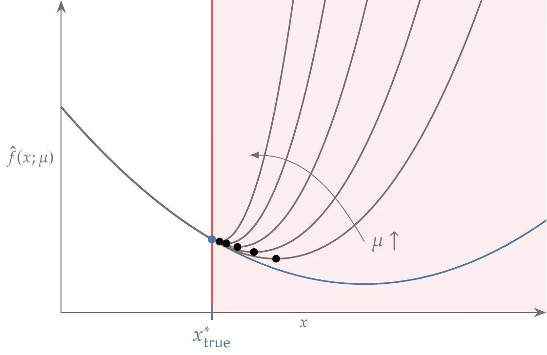
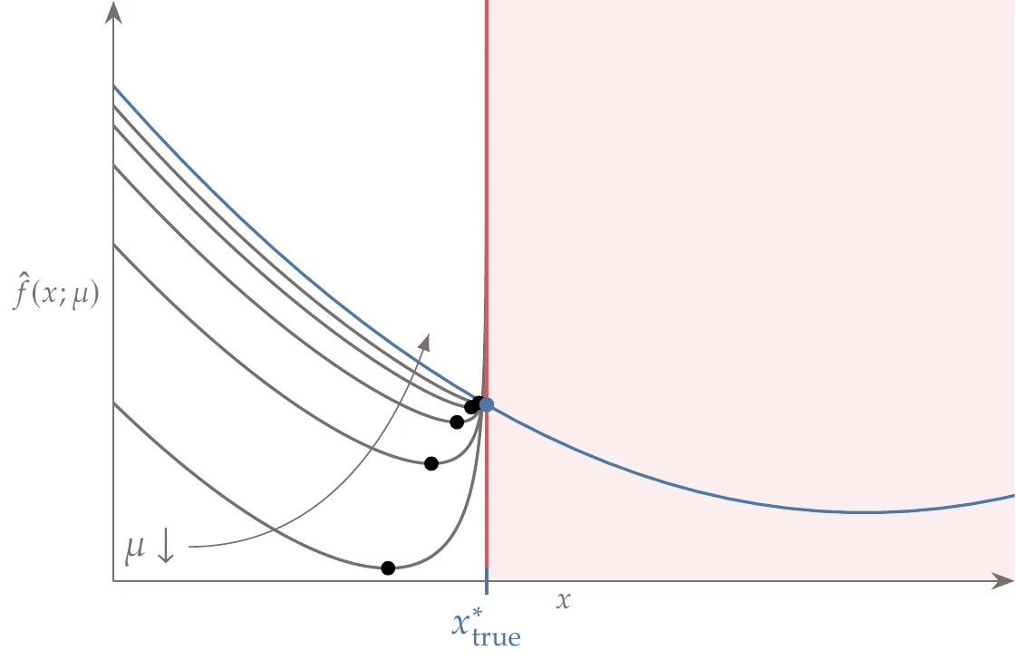
Like exterior penalty methods, interior penalty methods must also solve a sequence of unconstrained problems but with μ→0 (see Algorithm 5.3). As the penalty parameter decreases, the region across which the penalty acts decreases, as shown in Figure 5.35.
Figure 5.35:Logarithmic barrier penalty for an inequality constrained problem. The minimum of the penalized function (black circles) approaches the true constrained minimum (blue circle) as the penalty parameter μ decreases.
The methodology is the same as is described in Algorithm 5.1 but with a decreasing penalty parameter. One major weakness of the method is that the penalty function is not defined for infeasible points, so a feasible starting point must be provided. For some problems, providing a feasible starting point may be difficult or practically impossible.
The optimization must be safeguarded to prevent the algorithm from becoming infeasible when starting from a feasible point. This can be achieved by checking the constraints values during the line search and backtracking if any of them is greater than or equal to zero. Multiple backtracking iterations might be required.
Like exterior penalty methods, the Hessian for interior penalty methods becomes increasingly ill-conditioned as the penalty parameter tends to zero.8 There are augmented and modified barrier approaches that can avoid the ill-conditioning issue (and other methods that remain ill-conditioned but can still be solved reliably, albeit inefficiently).9 However, these methods have been superseded by the modern interior-point methods discussed in Section 5.6, so we do not elaborate on further improvements to classical penalty methods.
SQP is the first of the modern constrained optimization methods we discuss. SQP is not a single algorithm; instead, it is a conceptual method from which various specific algorithms are derived. We present the basic method but mention only a few of the many details needed for robust practical implementations. We begin with equality constrained SQP and then add inequality constraints.
To derive the SQP method, we start with the KKT conditions for this problem and treat them as equation residuals that need to be solved. Recall that the Lagrangian (Equation 5.12) is
Differentiating this function with respect to the design variables and Lagrange multipliers and setting the derivatives to zero, we get the KKT conditions,
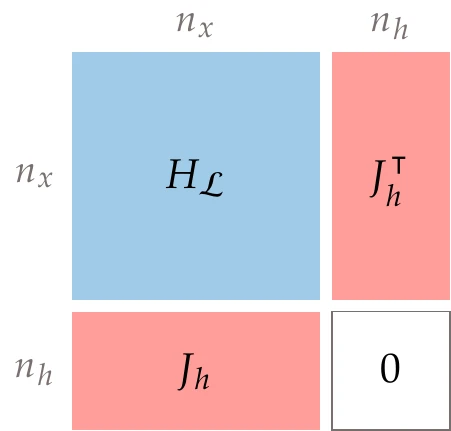
The shape of the matrix and its blocks are as shown in Figure 5.37. We solve a sequence of these problems to converge to the optimal design variables and the corresponding optimal Lagrange multipliers. At each iteration, we update the design variables and Lagrange multipliers as follows:
The inclusion of αk suggests that we do not automatically accept the Newton step (which corresponds to α=1) but instead perform a line search as previously described in Section 4.3. The function used in the line search needs some modification, as discussed later in this section.
SQP can be derived in an alternative way that leads to different insights. This alternate approach requires an understanding of quadratic programming (QP), which is discussed in more detail in Section 11.3 but briefly described here. A QP problem is an optimization problem with a quadratic objective and linear constraints. In a general form, we can express any equality constrained QP as
The constraint is a matrix equation that represents multiple linear equality constraints—one for every row in A. We can solve this optimization problem analytically from the optimality conditions. First, we form the Lagrangian:
This is like the procedure we used in solving the KKT conditions, except that these are linear equations, so we can solve them directly without any iteration. As in the unconstrained case, finding the minimum of a quadratic objective results in a system of linear equations.
As long as Q is positive definite, then the linear system always has a solution, and it is the global minimum of the QP.[11]The ease with which a QP can be solved provides a strong motivation for SQP. For a general constrained problem, we can make a local QP approximation of the nonlinear model, solve the QP, and repeat this process until convergence. This method involves iteratively solving a sequence of quadratic programming problems, hence the name sequential quadratic programming.
To form the QP, we use a local quadratic approximation of the Lagrangian (removing the constant term because it does not change the solution) and a linear approximation of the constraints for some step p near our current point. In other words, we locally approximate the problem as the following QP:
which is the same linear system we found from applying Newton’s method to the KKT conditions (Equation 5.62).
This derivation relies on the somewhat arbitrary choices of choosing a QP as the subproblem and using an approximation of the Lagrangian with constraints (rather than an approximation of the objective with constraints or an approximation of the Lagrangian with no constraints).[12] Nevertheless, it is helpful to conceptualize the method as solving a sequence of QPs. This concept will motivate the solution process once we add inequality constraints.
Introducing inequality constraints adds complications. For inequality constraints, we cannot solve the KKT conditions directly as we could for equality constraints. This is because the KKT conditions include the complementary slackness conditions σjgj=0, which we cannot solve directly. Even though the number of equations in the KKT conditions is equal to the number of unknowns, the complementary conditions do not provide complete information (they just state that each constraint is either active or inactive). Suppose we knew which of the inequality constraints were active (gj=0) and which were inactive (σj=0) at the optimum. Then, we could use the same approach outlined in the previous section, treating the active constraints as equality constraints and ignoring the inactive constraints. Unfortunately, we do not know which constraints are active at the optimum beforehand in general. Finding which constraints are active in an iterative way is challenging because we would have to try all possible combinations of active constraints. This is intractable if there are many constraints.
A common approach to handling inequality constraints is to use an active-set method. The active set is the set of constraints that are active at the optimum (the only ones we ultimately need to enforce). Although the actual active set is unknown until the solution is found, we can estimate this set at each iteration. This subset of potentially active constraints is called the working set.
The working set is then updated at each iteration.
Similar to the SQP developed in the previous section for equality constraints, we can create an algorithm based on solving a sequence of QPs that linearize the constraints.[13] We extend the equality constrained QP (Equation 5.69) to include the inequality constraints as follows:
The determination of the working set could happen in the inner loop, that is, as part of the inequality constrained QP subproblem (Equation 5.76). Alternatively, we could choose a working set in the outer loop and then solve the QP subproblem with only equality constraints (Equation 5.69), where the working-set constraints would be posed as equalities. The former approach is more common and is discussed here. In that case, we need consider only the active-set problem in the context of a QP. Many variations on active-set methods exist; we outline just one such approach based on a binding-direction method.
The general QP problem we need to solve is as follows:
We assume that Q is positive definite so that this problem is convex. Here, Q corresponds to the Lagrangian Hessian. Using an appropriate quasi-Newton approximation (which we will discuss in Section 5.5.4) ensures a positive definite Lagrangian Hessian approximation.
Consider iteration k in an SQP algorithm that handles inequality constraints. At the end of the previous iteration, we have a design point xk and a working set Wk. The working set in this approach is a set of row indices corresponding to the subset of inequality constraints that are active at xk.[14]Then, we consider the corresponding inequality constraints to be equalities, and we write:
where Cw and dw correspond to the rows of the inequality constraints specified in the working set.
The constraints in the working set, combined with the equality constraints, must be linearly independent. Thus, we cannot include more working-set constraints (plus equality constraints) than design variables.
Although the active set is unique, there can be multiple valid choices for the working set.
Assume, for the moment, that the working set does not change at nearby points (i.e., we ignore the constraints outside the working set). We seek a step p to update the design variables as follows: xk+1=xk+p. We find p by solving the following simplified QP that considers only the working set:
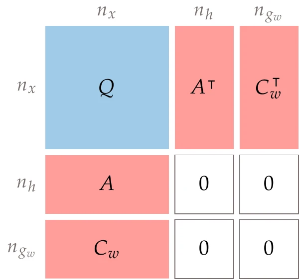
We solve this QP by varying p, so after multiplying out the terms in the objective, we can ignore the terms that do not depend on p. We can also simplify the constraints because we know the constraints were satisfied at the previous iteration (i.e., Axk+b=0 and Cwxk+dw=0). The simplified problem is as follows:
Figure 5.39 shows the structure of the matrix in this linear system.
Let us consider the case where the solution of this linear system is nonzero. Solving the KKT conditions in Equation 5.80 ensures that all the constraints in the working set are still satisfied at xk+p. Still, there is no guarantee that the step does not violate some of the constraints outside of our working set. Suppose that Cn and dn define the constraints outside of the working set. If
We cannot take the full step (α=1), but we would like to take as large a step as possible while still keeping all the constraints feasible.
Let us consider how to determine the appropriate step size, α. Substituting the step update (Equation 5.84) into the equality constraints, we obtain the following:
We know that Axk+b=0 from solving the problem at the previous iteration. Also, we just solved p under the condition that Ap=0. Therefore, the equality constraints (Equation 5.85) remain satisfied for any choice of α. By the same logic, the constraints in our working set remain satisfied for any choice of α as well.
Now let us consider the constraints that are not in the working set.
We denote ci as row i of the matrix Cn (associated with the inequality constraints outside of the working set). If these constraints are to remain satisfied, we require
We do not divide through by ci⊺p yet because the direction of the inequality would change depending on its sign. We consider the two possibilities separately. Because the QP constraints were satisfied at the previous iteration, we know that ci⊺xk+di≤0 for all i. Thus, the right-hand side is always positive. If ci⊺p is negative, then the inequality will be satisfied for any choice of α. Alternatively, if ci⊺p is positive, we can rearrange Equation 5.87 to obtain the following:
This equation determines how large α can be without causing one of the constraints outside of the working set to become active. Because multiple constraints may become active, we have to evaluate α for each one and choose the smallest α among all constraints.
A constraint for which α<1 is said to be blocking. In other words, if we had included that constraint in our working set before solving the QP, it would have changed the solution. We add one of the blocking constraints to the working set, and proceed to the next iteration.[15]Now consider the case where the solution to Equation 5.81 is p=0. If all inequality constraint Lagrange multipliers are positive (σi>0), the KKT conditions are satisfied and we have solved the original inequality constrained QP. If one or more σi values are negative, additional iterations are needed. We find the σi value that is most negative, remove constraint i from the working set, and proceed to the next iteration.
As noted previously, all the constraints in the reduced QP (the equality constraints plus all working-set constraints) must be linearly independent and thus [ACw]⊺ has full row rank. Otherwise, there would be no solution to Equation 5.81. Therefore, the starting working set might not include all active constraints at x0 and must instead contain only a subset, such that linear independence is maintained.
Similarly, when adding a blocking constraint to the working set, we must again check for linear independence. At a minimum, we need to ensure that the length of the working set does not exceed nx. The complete algorithm for solving an inequality constrained QP is shown in Algorithm 5.4.
Because SQP solves a sequence of QPs, an effective approach is to use the optimal x and active set from the previous QP as the starting point and working set for the next QP. The algorithm outlined in this section requires both a feasible starting point and a working set of linearly independent constraints. Although the previous starting point and working set usually satisfy these conditions, this is not guaranteed, and adjustments may be necessary.
Algorithms to determine a feasible point are widely used (often by solving a linear programming problem). There are also algorithms to remove or add to the constraint matrix as needed to ensure full rank.12
Similar to what we did in unconstrained optimization, we do not directly accept the step p returned from solving the subproblem (Equation 5.62 or Equation 5.76). Instead, we use p as the first step length in a line search.
In the line search for unconstrained problems (Section 4.3), determining if a point was good enough to terminate the search was based solely on comparing the objective function value (and the slope when enforcing the strong Wolfe conditions). For constrained optimization, we need to make some modifications to these methods and criteria.
In constrained optimization, objective function decrease and feasibility often compete with each other. During a line search, a new point may decrease the objective but increase the infeasibility, or it may decrease the infeasibility but increase the objective. We need to take these two metrics into account to determine the line search termination criterion.
The Lagrangian is a function that accounts for the two metrics. However, at a given iteration, we only have an estimate of the Lagrange multipliers, which can be inaccurate.
One way to combine the objective value with the constraints in a line search is to use merit functions, which are similar to the penalty functions introduced in Section 5.4. Common merit functions include functions that use the norm of constraint violations:
Like penalty functions, one downside of merit functions is that it is challenging to choose a suitable value for the penalty parameter μ. This parameter needs to be large to ensure feasibility. However, if it is too large, a full Newton step might not be permitted. This might slow the convergence unnecessarily. Using the augmented Lagrangian can help, as discussed in Section 5.4.1. However, there are specific techniques used in SQP line searches and various safeguarding techniques needed for robustness.
Filter methods are an alternative to using penalty-based methods in a line search.13 Filter methods interfere less with the full Newton step and are effective for both SQP and interior-point methods (which are introduced in Section 5.6).1415 The approach is based on concepts from multiobjective optimization, which is the subject of Chapter 9. In the filter method, there are two objectives: decrease the objective function and decrease infeasibility. A point is said to dominate another if its objective is lower and the sum of its constraint violations is lower. The filter consists of all the points that have been found to be non-dominated in the line searches so far. The line search terminates when it finds a point that is not dominated by any point in the current filter. That new point is then added to the filter, and any points that it dominates are removed from the filter.[16]This is only the basic concept. Robust implementation of a filter method requires imposing sufficient decrease conditions, not unlike those in the unconstrained case, and several other modifications. Fletcher et al. (2006) provide more details on filter methods.
In the discussion of the SQP method so far, we have assumed that we have the Hessian of the Lagrangian HL. Similar to the unconstrained optimization case, the Hessian might not be available or be too expensive to compute. Therefore, it is desirable to use a quasi-Newton approach that approximates the Hessian, as we did in Section 4.4.4.
The difference now is that we need an approximation of the Lagrangian Hessian instead of the objective function Hessian. We denote this approximation at iteration k as H~Lk.
Similar to the unconstrained case, we can approximate H~Lk using the gradients of the Lagrangian and a quasi-Newton update, such as the Broyden–Fletcher–Goldfarb–Shanno (BFGS) update.
Unlike in unconstrained optimization, we do not want the inverse of the Hessian directly. Therefore, we use the version of the BFGS formula that computes the Hessian (Equation 4.87):
The step in the design variable space, sk, is the step that resulted from the latest line search. The Lagrange multiplier is fixed to the latest value when approximating the curvature of the Lagrangian because we only need the curvature in the space of the design variables.
Recall that for the QP problem (Equation 5.76) to have a solution, H~Lk must be positive definite. To ensure a positive definite approximation, we can use a damped BFGS update.16[17]
This method replaces y with a new vector r, defined as
which can range from 0 to 1. We then use the same BFGS update formula (Equation 5.91), except that we replace each yk with rk.
To better understand this update, let us consider the two extremes for θ. If θk=0, then Equation 5.93 in combination with Equation 5.91 yields H~Lk+1=H~Lk; that is, the Hessian approximation is unmodified. At the other extreme, θk=1 yields the full BFGS update formula (rk is set to yk). Thus, the parameter θk provides a linear weighting between keeping the current Hessian approximation and using the full BFGS update.
The definition of θk (Equation 5.94) ensures that H~Lk+1 stays close enough to H~Lk and remains positive definite. The damping is activated when the predicted curvature in the new latest step is below one-fifth of the curvature predicted by the latest approximate Hessian. This could happen when the function is flattening or when the curvature becomes negative.
We now put together the various pieces in a high-level description of SQP with quasi-Newton approximations in Algorithm 5.5.[18] For the convergence criterion, we can use an infinity norm of the KKT system residual vector. For better control over the convergence, we can consider two separate tolerances: one for the norm of the optimality and another for the norm of the feasibility. For problems that only have equality constraints, we can solve the corresponding QP (Equation 5.62) instead.
Interior-point methods use concepts from both SQP and interior penalty methods.[19]These methods form an objective similar to the interior penalty but with the key difference that instead of penalizing the constraints directly, they add slack variables to the set of optimization variables and penalize the slack variables. The resulting formulation is as follows:
This formulation turns the inequality constraints into equality constraints and thus avoids the combinatorial problem.
Similar to SQP, we apply Newton’s method to solve for the KKT conditions. However, instead of solving the KKT conditions of the original problem (Equation 5.59), we solve the KKT conditions of the interior-point formulation (Equation 5.95).
These slack variables in Equation 5.95 do not need to be squared, as was done in deriving the KKT conditions, because the logarithm is only defined for positive s values and acts as a barrier preventing negative values of s (although we need to prevent the line search from producing negative s values, as discussed later). Because s is always positive, that means that g(x∗)<0 at the solution, which satisfies the inequality constraints.
Like penalty method formulations, the interior-point formulation (Equation 5.95) is only equivalent to the original constrained problem in the limit, as μb→0. Thus, as in the penalty methods, we need to solve a sequence of solutions to this problem where μb approaches zero.
where lns is an ng-vector whose components are the logarithms of each component of s, and e=[1,…,1] is an ng-vector of 1s introduced to express the sum in vector form. By taking derivatives with respect to x, λ, σ, and s, we derive the KKT conditions for this problem as
where S is a diagonal matrix whose diagonal entries are given by the slack variable vector, and therefore Skk−1=1/sk. The result is a set of nx+nh+2ng equations and the same number of variables.
To get a system of equations that is more favorable for Newton’s method, we multiply the last equation by S to obtain
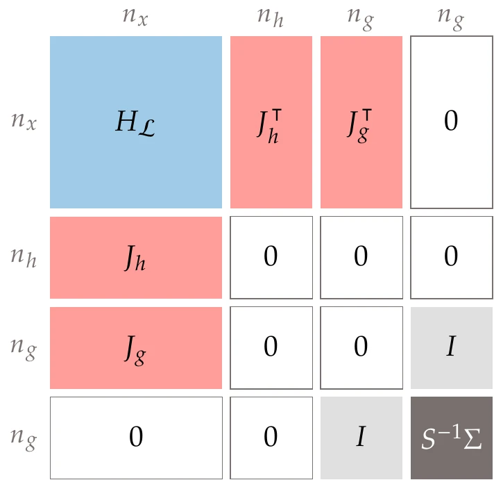
We now have a set of residual equations to which we can apply Newton’s method, just like we did for SQP. Taking the Jacobian of the residuals in Equation 5.98, we obtain the linear system
where Σ is a diagonal matrix whose entries are given by σ, and I is the identity matrix. For numerical efficiency, we make the matrix symmetric by multiplying the last equation by S−1 to get the symmetric linear system, as follows:
The advantage of this equivalent system is that we can use a linear solver specialized for symmetric matrices, which is more efficient than a solver for general linear systems.
If we had applied Newton’s method to the original KKT system (Equation 5.97) and then made it symmetric, we would have obtained a term with S−2, which would make the system more challenging than with the S−1 term in Equation 5.100. Figure 5.46 shows the structure and block sizes of the matrix.
We can reuse many of the concepts covered under SQP, including quasi-Newton estimates of the Lagrangian Hessian and line searches with merit functions or filters. The merit function would usually be modified to a form more consistent with the formulation used in Equation 5.95. For example, we could write a merit function as follows:
where μb is the barrier parameter from Equation 5.95, and μp is the penalty parameter. Additionally, we must enforce an αmax in the line search so that the implicit constraint on s>0 remains enforced. The maximum allowed step size can be computed prior to the line search because we know the value of s and ps and require that
where τ is a small value (e.g., τ=0.005). The maximum step size is the smallest positive value that satisfies this equation for all entries in s. A possible algorithm for determining the maximum step size for feasibility is shown in Algorithm 5.6.
The line search typically uses a simple backtracking approach because we must enforce a maximum step length. After the line search, we can update x and s as follows:
The Lagrange multipliers σ must also remain positive, so the procedure in Algorithm 5.6 is repeated for σ to find the maximum step length for the Lagrange multipliers ασ. Enforcing a maximum step size for Lagrange multiplier updates was not necessary for the SQP method because the QP subproblem handled the enforcement of nonnegative Lagrange multipliers. We then update both sets of Lagrange multipliers using this step size:
where ρ is typically around 0.2. Better methods are adaptive based on how well the optimizer is progressing. There are other implementation details for improving robustness that can be found in the literature.2223
The steps for a basic interior-point method are detailed in Algorithm 5.7.[20]
This version focuses on a line search approach, but there are variations of interior-point methods that use the trust-region approach.
Both interior-point methods and SQP are considered state-of-the-art approaches for solving nonlinear constrained optimization problems. Each of these two methods has its strengths and weaknesses. The KKT system structure is identical at each iteration for interior-point methods, so we can exploit this structure for improved computational efficiency. SQP is not as amenable to this because changes in the working set cause the system’s structure to change between iterations. The downside of the interior-point structure is that turning all constraints into equalities means that all constraints must be included at every iteration, even if they are inactive. In contrast, active-set SQP only needs to consider a subset of the constraints, reducing the subproblem size.
Active-set SQP methods are generally more effective for medium-scale problems, whereas interior-point methods are more effective for large-scale problems.
Interior-point methods are usually more sensitive to the initial starting point and the scaling of the problem. Therefore, SQP methods are usually more suitable for solving sequences of warm-started problems.2511 These are just general guidelines; both approaches should be considered and tested for a given problem of interest.
As will be discussed in Chapter 6, some derivative computation methods are efficient for problems with many inputs and few outputs, and others are advantageous for problems with few inputs and many outputs. Thus, if we have many design variables and many constraints, there is no efficient way to compute the required constraint Jacobian.
One workaround is to aggregate the constraints and solve the optimization problem with a new set of constraints. Each aggregation would have the form
where gˉ is a scalar, and g is the vector of constraints we want to aggregate. One of the properties we want for the aggregation function is that if any of the original constraints are violated, then gˉ>0.
One way to aggregate constraints would be to define the aggregated constraint function as the maximum of all constraints,
If max(g(x))≤0, then we know that all of components of g(x)≤0. However, the maximum function is not differentiable, so it is not desirable for gradient-based optimization.
In the rest of this section, we introduce several viable functions for constraint aggregation that are differentiable.
The Kreisselmeier–Steinhauser (KS) aggregation was one of the first aggregation functions proposed for optimization and is defined as follows:26
where ρ is an aggregation factor that determines how close this function is to the maximum function (Equation 5.110). As ρ→∞, gˉKS(ρ,g)→max(g). However, as ρ increases, the curvature of gˉ increases, which can cause ill-conditioning in the optimization.
The exponential function disproportionately weighs the higher positive values in the constraint vector, but it does so in a smooth way. Because the exponential function can easily result in overflow, it is preferable to use the alternate (but equivalent) form of the KS function,
The absolute value in this equation can be an issue if g can take both positive and negative values because the function is not differentiable in regions where g transitions from positive to negative.
A class of aggregation functions known as induced functions was designed to provide more accurate estimates of max(g) for a given value of ρ than the KS and induced norm functions.28 There are two main types of induced functions: one uses exponentials, and the other uses powers. The induced exponential function is given by
Most engineering design problems are constrained. When formulating a problem, practitioners should be critical of their choice of objective function and constraints. Metrics that should be constraints are often wrongly formulated as objectives. A constraint should not limit the design unnecessarily and should reflect the underlying physical reason for that constraint as much as possible.
The first-order optimality conditions for constrained problems—the KKT conditions—require the gradient of the objective to be a linear combination of the gradients of the constraints. This ensures that there is no feasible descent direction. Each constraint is associated with a Lagrange multiplier that quantifies how significant that constraint is at the optimum. For inequality constraints, a Lagrange multiplier that is zero means that the corresponding constraint is inactive. For inequality constraints, slack variables quantify how close a constraint is to becoming active; a slack variable that is zero means that the corresponding constraint is active. Lagrange multipliers and slack variables are unknowns that need to be solved together with the design variables. The complementary slackness condition introduces a combinatorial problem that is challenging to solve.
Penalty methods solve constrained problems by adding a metric to the objective function quantifying how much the constraints are violated. These methods are helpful as a conceptual model and are used in gradient-free optimization algorithms (Chapter 7). However, penalty methods only find approximate solutions and are subject to numerical issues when used with gradient-based optimization.
Methods based on the KKT conditions are preferable. The most widely used among such methods are SQP and interior-point methods. These methods apply Newton’s method to the KKT conditions. One primary difference between these two methods is in the treatment of inequality constraints. SQP methods distinguish between active and inactive constraints, treating potentially active constraints as equality constraints and ignoring the potentially inactive ones. Interior-point methods add slack variables to force all constraints to behave like equality constraints.
Despite our convention of reserving Greek symbols for scalars, we use λ to represent the nh-vector of Lagrange multipliers because it is common usage.
Farkas’ lemma has other applications beyond optimization and can be written in various equivalent forms. Using the statement by 3 we set A=Jg, x=−p, c=−∇f, and y=σ.
In practice, adding only one constraint to the working set at a time (or removing only one constraint in other steps described later) typically leads to faster convergence.
The damped BFGS update is not always the best approach. There are approaches built around other approximation methods, such as symmetric rank 1 (SR1).17 Limited-memory updates similar to L-BFGS (see Section 4.4.5) can be used when storing a dense Hessian for large problems is prohibitive.18
A few popular SQP implementations include SNOPT,12 Knitro,19 MATLAB’s fmincon, and SLSQP.20 The first three are commercial options, whereas SLSQP is open source. There are interfaces in different programming languages for these optimizers, including pyOptSparse (for SNOPT and SLSQP).21
The name interior point stems from early methods based on interior penalty methods that assumed that the initial point was feasible. However, modern interior-point methods can start with infeasible points.
IPOPT is an open-source nonlinear interior-point method.24 The commercial packages Knitro19 and fmincon mentioned earlier also include interior-point methods.
This is a well-known optimization problem formulated by 30 when he first proposed integrating numerical optimization with finite-element structural analysis.
Boyd, S. P., & Vandenberghe, L. (2004). Convex Optimization. Cambridge University Press.
Strang, G. (2006). Linear Algebra and its Applications (4th ed.). Cengage Learning.
Dax, A. (1997). Classroom note: An elementary proof of Farkas’ lemma. SIAM Review, 39(3), 503–507. 10.1137/S0036144594295502
Gill, P. E., Murray, W., Saunders, M. A., & Wright, M. H. (1986). Some theoretical properties of an augmented Lagrangian merit function [SOL 86-6R]. Systems Optimization Laboratory. https://apps.dtic.mil/sti/citations/ADA168503
Di Pillo, G., & Grippo, L. (1982). A new augmented Lagrangian function for inequality constraints in nonlinear programming problems. Journal of Optimization Theory and Applications, 36(4), 495–519. 10.1007/BF00940544
Birgin, E. G., Castillo, R. A., & MartÍnez, J. M. (2005). Numerical comparison of augmented Lagrangian algorithms for nonconvex problems. Computational Optimization and Applications, 31(1), 31–55. 10.1007/s10589-005-1066-7
Rockafellar, R. T. (1973). The multiplier method of Hestenes and Powell applied to convex programming. Journal of Optimization Theory and Applications, 12(6), 555–562. 10.1007/BF00934777
Murray, W. (1971). Analytical expressions for the eigenvalues and eigenvectors of the Hessian matrices of barrier and penalty functions. Journal of Optimization Theory and Applications, 7(3), 189–196. 10.1007/bf00932477
Forsgren, A., Gill, P. E., & Wright, M. H. (2002). Interior methods for nonlinear optimization. SIAM Review, 44(4), 525–597. 10.1137/s0036144502414942
Gill, P. E., & Wong, E. (2012). Sequential quadratic programming methods. In J. Lee & S. Leyffer (Eds.), Mixed Integer Nonlinear Programming (Vol. 154). Springer. 10.1007/978-1-4614-1927-3_6
Nocedal, J., & Wright, S. J. (2006). Numerical Optimization (2nd ed.). Springer. 10.1007/978-0-387-40065-5
Gill, P. E., Murray, W., & Saunders, M. A. (2005). SNOPT: An SQP algorithm for large-scale constrained optimization. SIAM Review, 47(1), 99–131. 10.1137/S0036144504446096
Fletcher, R., & Leyffer, S. (2002). Nonlinear programming without a penalty function. Mathematical Programming, 91(2), 239–269. 10.1007/s101070100244
Benson, H. Y., Vanderbei, R. J., & Shanno, D. F. (2002). Interior-point methods for nonconvex nonlinear programming: Filter methods and merit functions. Computational Optimization and Applications, 23(2), 257–272. 10.1023/a:1020533003783