Convex Optimization - Engineering Design Optimization

General nonlinear optimization problems are difficult to solve. Depending on the particular optimization algorithm, they may require tuning parameters, providing derivatives, adjusting scaling, and trying multiple starting points. Convex optimization problems do not have any of those issues and are thus easier to solve. The challenge is that these problems must meet strict requirements. Even for candidate problems with the potential to be convex, significant experience is usually needed to recognize and utilize techniques that reformulate the problems into an appropriate form.

11.1 Introduction¶

Convex optimization problems have desirable characteristics that make them more predictable and easier to solve. Because a convex problem has provably only one optimum, convex optimization methods always converge to the global minimum. Solving convex problems is straightforward and does not require a starting point, parameter tuning, or derivatives, and such problems scale well up to millions of design variables.1

All we need to solve a convex problem is to set it up appropriately; there is no need to worry about convergence, local optima, or noisy functions. Some convex problems are so straightforward that they are not recognized as an optimization problem and are just thought of as a function or operation. A familiar example of the latter is the linear-least-squares problem (described previously in Section 10.3.1 and revisited in a subsequent section).

Although these are desirable properties, the catch is that convex problems must satisfy strict requirements. Namely, the objective and all inequality constraints must be convex functions, and the equality constraints must be affine.^[1]A function $f$ is convex if

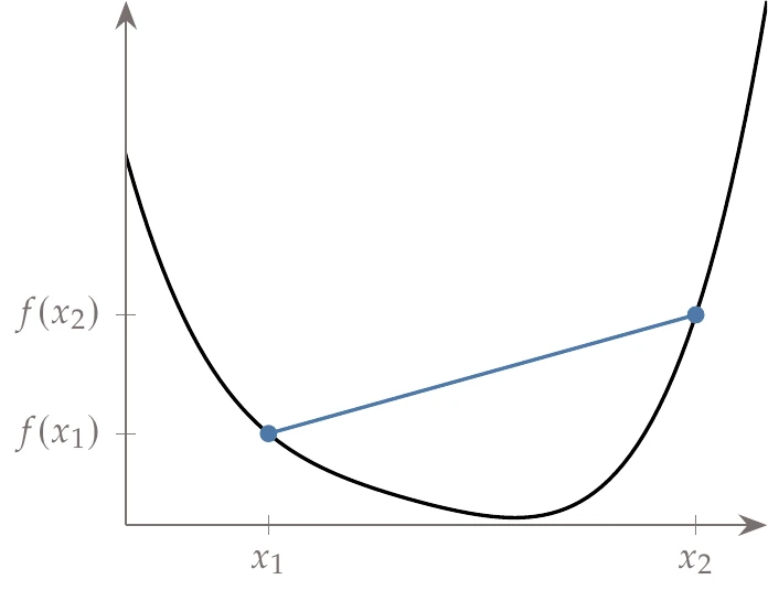
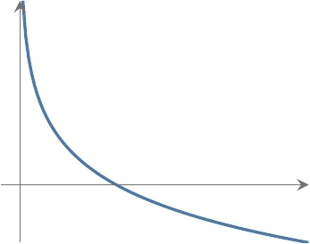
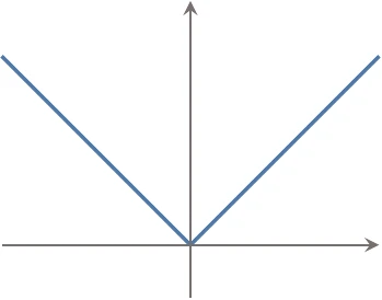
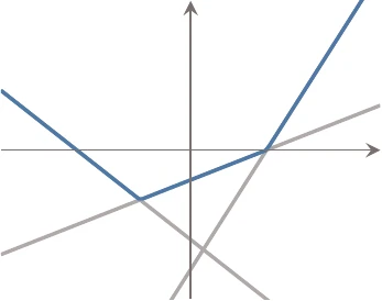
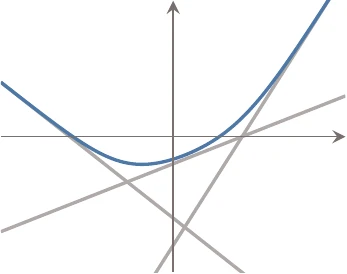
f \left( (1-\eta) x_1 + \eta x_2 \right) \le (1-\eta) f(x_1) + \eta f(x_2)

(11.1)

for all $x_1$ and $x_2$ in the domain, where $0 \le \eta \le 1$ . This requirement is illustrated in Figure 11.1 for the one-dimensional case. The right-hand side of the inequality is just the equation of a line from $f(x_1)$ to $f(x_2)$ (the blue line), whereas the left-hand side is the function $f(x)$ evaluated at all points between $x_1$ and $x_2$ (the black curve).

Figure 11.1:Convex function definition in the one-dimensional case: The function (black line) must be below a line that connects any two points in the domain (blue line).

The inequality says that the function must always be below a line joining any two points in the domain. Stated informally, a convex function looks something like a bowl.

Unfortunately, even these strict requirements are not enough. In general, we cannot identify a given problem as convex or take advantage of its structure to solve it efficiently and must therefore treat it as a general nonlinear problem. There are two approaches to taking advantage of convexity. The first one is to directly formulate the problem in a known convex form, such as a linear program or a quadratic program (discussed later in this chapter). The second option is to use disciplined convex optimization, a specific set of rules and mathematical functions that we can use to build up a convex problem. By following these rules, we can automatically translate the problem into an efficiently solvable form.

Although both of these approaches are straightforward to apply, they also expose the main weakness of these methods: we need to express the objective and inequality constraints using only these elementary functions and operations. In most cases, this requirement means that the model must be simplified.

Often, a problem is not directly expressed in a convex form, and a combination of experience and creativity is needed to reformulate the problem in an equivalent manner that is convex.

Simplifying models usually results in a fidelity reduction. This is less problematic for optimization problems intended to be solved repeatedly, such as in optimal control and machine learning, which are domains in which convex optimization is heavily used. In these cases, simplification by local linearization, for example, is less problematic because the linearization can be updated in the next time step. However, this fidelity reduction is problematic for design applications.

In design scenarios, the optimization is performed once, and the design cannot continue to be updated after it is created. For this reason, convex optimization is less frequently used for design applications, except for some limited uses in geometric programming, a topic discussed in more detail in Section 11.6.

This chapter just introduces convex optimization and is not a replacement for more comprehensive textbooks on the topic.^[2] We focus on understanding what convex optimization is useful for and describing the most widely used forms.

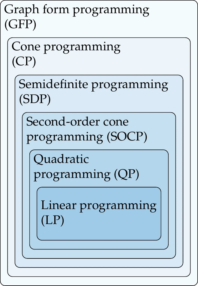
The known categories of convex optimization problems include linear programming, quadratic programming, second-order cone programming, semidefinite programming, cone programming, and graph form programming. Each of these categories is a subset of the next (Figure 11.2).^[3]

We focus on the first three because they are the most widely used, including in other chapters in this book. The latter three forms are less frequently formulated directly. Instead, users apply elementary functions and operations and the rules specified by disciplined convex programming, and a software tool transforms the problem into a suitable conic form that can be solved. Section 11.5 describes this procedure.

Figure 11.2:Relationship between various convex optimization problems.

After covering the three main categories of convex optimization problems, we discuss geometric programming. Geometric programming problems are not convex, but with a change of variables, they can be transformed into an equivalent convex form, thus extending the types of problems that can be solved with convex optimization.

11.2 Linear Programming¶

A linear program (LP) is an optimization problem with a linear objective and linear constraints and can be written as

\begin{aligned} \underset{x}{\text{minimize}} &\quad f^\intercal x\\ \text{subject to} &\quad A x + b = 0\\ &\quad Cx + d \le 0 \, , \end{aligned}

(11.2)

where $f$ , $b$ , and $d$ are vectors and $A$ and $C$ are matrices. All LPs are convex.

Example 11.1 (Formulating a linear programming problem)

Suppose we are shopping and want to find how best to meet our nutritional needs for the lowest cost. We enumerate all the food options and use the variable $x_j$ to represent how much of food $j$ we purchase. The parameter $c_j$ is the cost of a unit amount of food $j$ . The parameter $N_{ij}$ is the amount of nutrient $i$ contained in a unit amount of food $j$ . We need to make sure we have at least $r_i$ of nutrient $i$ to meet our dietary requirements. We can now formulate the cost objective as

\underset{x}{\text{minimize}} \quad \sum_j c_j x_j = c^\intercal x \, .

To meet the nutritional requirement of nutrient $i$ , we need to satisfy

\sum_j N_{ij} x_j \ge r_i \Rightarrow N x \ge r \, .

Finally, we cannot purchase a negative amount of food, so $x \ge 0$ . The objective and all of the constraints are linear in $x$ , so this is an LP (where $f \equiv c$ , $C \equiv -N$ , $d \equiv r$ in Equation 11.2). We do not need to artificially restrict which foods we include in our initial list of possibilities. The formulation allows the optimizer to select a given food item $x_i$ to be zero (i.e., do not purchase any of that food item), according to what is optimal.

As a concrete example, consider a simplified version (and a reductionist view of nutrition) with 10 food options and three nutrients with the amounts listed in the following table.

Food	Cost	Nutrient 1	Nutrient 2	Nutrient 3
A	0.46	0.56	0.29	0.48
B	0.54	0.84	0.98	0.55
C	0.40	0.23	0.36	0.78
D	0.39	0.48	0.14	0.59
E	0.49	0.05	0.26	0.79
F	0.03	0.69	0.41	0.84
G	0.66	0.87	0.87	0.01
H	0.26	0.85	0.97	0.77
I	0.05	0.88	0.13	0.13
J	0.60	0.62	0.69	0.10

If the amount of each food is $x$ , the cost column is $c$ , and the nutrient columns are $n_1, n_2$ , and $n_3$ , we can formulate the LP as

\begin{aligned} \underset{x}{\text{minimize}} &\quad c^\intercal x\\ \text{subject to} &\quad 5 \le n_1^\intercal x \le 8\\ &\quad 7 \le n_2^\intercal x\\ &\quad 1 \le n_3^\intercal x \le 10\\ &\quad x \le 4 \, . \end{aligned}

The last constraint ensures that we do not overeat any one item and get tired of it. LP solvers are widely available, and because the inputs of an LP are just a table of numbers some solvers do not even require a programming language. The solution for this problem is

x = [0, 1.43, 0, 0, 0, 4.00, 0, 4.00, 0.73, 0] \, ,

suggesting that our optimal diet consists of items B, F, H, and I in the proportions shown here. The solution reached the upper limit for nutrient 1 and the lower limit for nutrient 2.

LPs frequently occur with allocation or assignment problems, such as choosing an optimal portfolio of stocks, deciding what mix of products to build, deciding what tasks should be assigned to each worker, or determining which goods to ship to which locations. These types of problems frequently occur in domains such as operations research, finance, supply chain management, and transportation.^[4]A common consideration with LPs is whether or not the variables should be discrete. In Example 11.1, $x_i$ is a continuous variable, and purchasing fractional amounts of food may or may not be possible, depending on the type of food. Suppose we were performing an optimal stock allocation. In that case, we can purchase fractional amounts of stock. However, if we were optimizing how much of each product to manufacture, it might not be feasible to build 32.4 products. In these cases, we need to restrict the variables to be integers using integer constraints. These types of problems require discrete optimization algorithms, which are covered in Chapter 8. Specifically, we discussed a mixed-integer LP in (Section 8.3).

11.3 Quadratic Programming¶

A quadratic program (QP) has a quadratic objective and linear constraints. Quadratic programming was introduced in Section 5.5 in the context of sequential quadratic programming. A general QP can be expressed as follows:

\begin{aligned} \underset{x}{\text{minimize}} &\quad \frac{1}{2}x^\intercal Q x + f^\intercal x\\ \text{subject to} &\quad Ax + b = 0\\ &\quad C x + d \le 0 \,. \end{aligned}

(11.3)

A QP is only convex if the matrix $Q$ is positive semidefinite. If $Q = 0$ , a QP reduces to an LP.

One of the most common QP examples is least squares regression, which was discussed previously in Section 10.3.1 and is used in many applications such as data fitting.

The linear least-squares problem has an analytic solution if $A$ has full rank, so the machinery of a QP is not necessary. However, we can add constraints in QP form to solve constrained least squares problems, which do not have analytic solutions in general.

Example 11.2 (A constrained least squares QP)

The left pane of Figure 11.3 shows some example data that are both noisy and biased relative to the true (but unknown) underlying curve, represented as a dashed line. Given the data points, we would like to estimate the underlying functional relationship. We assume that the relationship is cubic and write it as

y(x) = a_1 x^3 + a_2 x^2 + a_3 x + a_4 \, .

We need to estimate the coefficients $a_1, \ldots, a_4$ . As discussed previously, this can be posed as a QP problem or, even more simply, as an analytic problem. The middle pane of Figure 11.3 shows the resulting least squares fit.

Figure 11.3:True function on the left, least squares in the middle, and constrained least squares on the right.

Suppose that we know the upper bound of the function value based on measurements or additional data at a few locations. In this example, assume that we know that $f(-2) \le -2$ , $f(0) \le 4$ , and $f(2) \le 26$ . These requirements can be posed as linear constraints:

\begin{bmatrix} (-2)^3 & (-2)^2 & -2 & 1 \\ 0 & 0 & 0 & 1 \\ 2^3 & 2^2 & 2 & 1 \\ \end{bmatrix} \begin{bmatrix} a_1 \\ a_2 \\ a_3 \\ a_4 \end{bmatrix} \le \begin{bmatrix} -2 \\ 4 \\ 26 \end{bmatrix} \, .

After adding these linear constraints and retaining a quadratic objective (the sum of the squared error), the resulting problem is still a QP. The resulting solution is shown in the right pane of Figure 11.3, which results in a much more accurate fit.

Example 11.3 (Linear-quadratic regulator (LQR) controller)

Another common example of a QP occurs in optimal control. Consider the following discrete-time linear dynamic system:

x_{t+1} = A x_t + B u_t \, ,

where $x_t$ is the deviation from a desired state at time $t$ (e.g., the positions and velocities of an aircraft), and $u_t$ represents the control inputs that we want to optimize (e.g., control surface deflections). This dynamic equation can be used as a set of linear constraints in an optimization problem, but we must decide on an objective.

We would like to have small $x_t$ because that would mean reducing the error in our desired state quickly, but we would also like to have small $u_t$ because small control inputs require less energy. These are competing objectives, where a small control input will take longer to minimize error in a state, and vice versa.

One way to express this objective is as a quadratic function,

\underset{x,u}{\text{minimize}} \quad \frac{1}{2}\sum_{t = 0}^n \left(x_t^\intercal Q x_t + u_t^\intercal R u_t\right) \, ,

where the weights in $Q$ and $R$ reflect our preferences on how important it is to have a small state error versus small control inputs.^[5]This function has a form similar to kinetic energy, and the LQR problem could be thought of as determining the control inputs that minimize the energy expended, subject to the vehicle dynamics. This choice of the objective function was intentional because the problem is a convex QP (as long as we choose positive weights). Because it is convex, this problem can be solved reliably and efficiently, which are necessary conditions for a robust control law.

11.4 Second-Order Cone Programming¶

A second-order cone program (SOCP) has a linear objective and a second-order cone constraint:

\begin{aligned} \underset{x}{\text{minimize}} &\quad f^\intercal x\\ \text{subject to} &\quad \|A_i x + b_i\|_2 \le c_i^\intercal x + d_i\\ &\quad Gx + h = 0 \, . \end{aligned}

(11.4)

If $A_i = 0$ , then this form reduces to an LP.

One useful subset of SOCP is a quadratically constrained quadratic program (QCQP). A QCQP is the same as a QP but has quadratic inequality constraints instead of linear ones, that is,

\begin{aligned} \underset{x}{\text{minimize}} &\quad \frac{1}{2}x^\intercal Q x + f^\intercal x\\ \text{subject to} &\quad A x + b = 0 \\ &\quad \frac{1}{2}x^\intercal R_i x + c_i^\intercal x + d_i \le 0 \text{ for } i = 1, \ldots, m \, , \end{aligned}

(11.5)

where $Q$ and $R$ must be positive semidefinite for the QCQP to be convex. A QCQP reduces to a QP if $R = 0$ . We formulated QCQPs when solving trust-region problems in Section 4.5. However, for trust-region problems, only an approximate solution method is typically used.

Every QCQP can be expressed as an SOCP (although not vice versa). The QCQP in Equation 11.5 can be written in the equivalent form,

\begin{aligned} \underset{x,\beta}{\text{minimize}} &\quad \beta \\ \text{subject to} &\quad \|Fx + g\|_2 \le \beta\\ &\quad A x + b = 0\\ &\quad \|G_i x + h_i\|_2 \le 0 \, . \end{aligned}

(11.6)

If we square both sides of the first and last constraints, this formulation is exactly equivalent to the QCQP where $Q = 2 F^\intercal F$ , $f = 2 F^\intercal g$ , $R_i = 2 G_i^\intercal G_i$ , $c_i = 2 G_i^\intercal h_i$ , and $d_i = h_i^\intercal h_i$ . The matrices $F$ and $G_i$ are the square roots of the matrices $Q$ and $R_i$ , respectively (divided by 2), and would be computed from a factorization.

11.5 Disciplined Convex Optimization¶

Disciplined convex optimization builds convex problems using a specific set of rules and mathematical functions. By following this set of rules, the problem can be translated automatically into a conic form that we can efficiently solve using convex optimization algorithms.5 Table 1 shows several examples of convex functions that can be used to build convex problems. Notice that not all functions are continuously differentiable because this is not a requirement of convexity.

A disciplined convex problem can be formulated using any of these functions for the objective and inequality constraints. We can also use various operations that preserve convexity to build up more complex functions. Some of the more common operations are as follows:

Multiplying a convex function by a positive constant
Adding convex functions
Composing a convex function with an affine function (i.e., if $f(x)$ is convex, then $f(Ax + b)$ is also convex)
Taking the maximum of two convex functions

Although these functions and operations greatly expand the types of convex problems that we can solve beyond LPs and QPs, they are still restrictive within the broader scope of nonlinear optimization. Still, for objectives and constraints that require only simple mathematical expressions, there is the possibility that the problem can be posed as a disciplined convex optimization problem.

The original expression of a problem is often not convex but can be made convex through a transformation to a mathematically equivalent problem. These transformation techniques include implementing a change of variables, adding slack variables, or expressing the objective in a different form. Successfully recognizing and applying these techniques is a skill requiring experience.

Example 11.4 (A supervised learning classification problem)

A classification problem seeks to determine a decision boundary between two sets of data. For example, given a large set of engineering parts, each associated with a label identifying whether it was defective or not, we would like to determine an optimal set of parameters that allow us to predict whether a new part will be defective or not. First, we have to decide on a set of features, or properties that we use to characterize each data point. For an engineering part, for example, these features might include dimensions, weights and moments of inertia, or surface finish.

If the data are separable, we could find a hyperplane,

f(x) = a^\intercal x + \beta\, ,

that separates the two data sets, or in other words, a function that classifies the objects. For example, if we call one data set $y_i, \text{ for } i = 1 \ldots n_y$ , and the other $z_i, \text{ for } i = 1 \ldots n_z$ , we need to satisfy the following constraints:

\begin{aligned} &a^\intercal y_i + \beta \ge \varepsilon\\ &a^\intercal z_i + \beta \le -\varepsilon\, , \end{aligned}

(11.7)

for some small tolerance $\varepsilon$ . In general, there are an infinite number of separating hyperplanes, so we seek the one that maximizes the distance between the points. However, such a problem is not yet well defined because we can multiply $a$ and $\beta$ in the previous equations by an arbitrary constant to achieve any separation we want, so we need to normalize or fix some reference dimension (only the ratio of the parameters matters in defining the hyperplane, not their absolute magnitudes). We define the optimization problem as follows:

\begin{aligned} \text{maximize} &\quad \gamma \\ \text{by varying} &\quad \gamma, a, \beta \\ \text{subject to} &\quad a^\intercal y_i + \beta \ge \gamma \text{ for } i = 1 \ldots n_y\\ &\quad a^\intercal z_j + \beta \le -\gamma \text{ for } j = 1, \ldots, n_z\\ &\quad \| a \| \le 1 \, . \end{aligned}

The last constraint provides a normalization to prevent the problem from being unbounded. This norm constraint is always active ( $\| a \| = 1$ ), but we express it as an inequality so that the problem remains convex (recall that equality constraints must be affine, but inequality constraints can be any convex function). The objective and inequality constraints are all convex functions, so we can solve it in a disciplined convex programming environment. Alternatively, in this case, we could employ a change of variables to put the problem in QP form if desired.

Figure 11.4:Two separable data sets are shown as points with two different colors. A classification boundary with maximum width is shown.

An example is shown in Figure 11.4 for data with two features for easy visualization. The middle line shows the separating hyperplane and the outer lines are a distance of $\gamma$ away, just passing through a data point from each set.

If the data are not completely separable, we need to modify our approach. Even if the data are separable, outliers may undesirably pull the hyperplane so that points are closer to the boundary than is necessary. To address these issues, we need to relax the constraints. As discussed, Equation 11.7 can always be multiplied by an arbitrary constant. Therefore, we can equivalently express the constraints as follows:

\begin{aligned} &a^\intercal y_i + \beta \ge 1\\ &a^\intercal z_j + \beta \le -1\, . \end{aligned}

To relax these constraints, we add nonnegative slack variables, $u_i$ and $v_j$ :

\begin{aligned} &a^\intercal y_i + \beta \ge 1 - u_i\\ &a^\intercal z_j + \beta \le -(1 - v_j)\, , \end{aligned}

where we seek to minimize the sum of the entries in $u$ and $v$ . If they sum to 0, we have the original constraints for a completely separable function. However, recall that we are interested in not just creating separation but also in maximizing the distance to the classification boundary. To accomplish this, we use a regularization approach where our two objectives include maximizing the distance from the boundary and maximizing the sum of the classification margins. The width between the two planes $a^\intercal x + \beta = 1$ and $a^\intercal x + \beta = -1$ is $2/\|a\|$ . Therefore, to maximize the separation distance, we minimize $\|a\|$ . The optimization problem is defined as follows:^[7]

\begin{aligned} \text{minimize} &\quad \|a\| + \omega \left(\sum_i u_i + \sum_j v_j\right) \\ \text{by varying} &\quad a, \beta, u, v\\ \text{subject to} &\quad a^\intercal y_i + \beta \ge (1 - u_i), & i = 1, \ldots, n_y\\ &\quad a^\intercal z_j + \beta \le -(1 - v_j), & j = 1, \ldots, n_z\\ &\quad u \ge 0 \\ &\quad v \ge 0 \, . \end{aligned}

Here, $\omega$ is a user-chosen weight reflecting a preference for the trade-offs in separation margin and stricter classification. The problem is still convex, and an example is shown in Figure 11.5 with a weight of $\omega = 1$ .

Figure 11.5:A classification boundary is shown for nonseparable data using a regularization approach.

The methodology can handle nonlinear classifiers by using a different form with kernel functions like those discussed in Section 10.4.

11.6 Geometric Programming¶

A geometric program (GP) is not convex but can be transformed into an equivalent convex problem. GPs are formulated using monomials and posynomials. A monomial is a function of the following form:

f(x) = c x_1^{a_1} x_2^{a_2} \cdots x_m^{a_m},

(11.8)

where $c > 0$ , and all $x_i > 0$ . A posynomial is a sum of monomials:

f(x) = \sum_{j=1}^n c_j x_1^{a_{1j}} x_2^{a_{2j}} \cdots x_m^{a_{mj}},

(11.9)

where all $c_j > 0$ .

A GP in standard form is written as follows:

\begin{aligned} \underset{x}{\text{minimize}} &\quad f_0(x)\\ \text{subject to} &\quad f_i(x) \le 1 \\ &\quad h_i(x) = 1 \, , \end{aligned}

(11.10)

where $f_i$ are posynomials, and $h_i$ are monomials. This problem does not fit into any of the convex optimization problems defined in the previous section, and it is not convex. This formulation is useful because we can convert it into an equivalent convex optimization problem.

First, we take the logarithm of the objective and of both sides of the constraints:

\begin{aligned} \underset{x}{\text{minimize}} &\quad \ln f_0(x)\\ \text{subject to} &\quad \ln f_i(x) \le 0 \\ &\quad \ln h_i(x) = 0 \, . \end{aligned}

(11.11)

Let us examine the equality constraints further. Recall that $h_i$ is a monomial, so writing one of the constraints explicitly results in the following form:

\ln \left(c x_1^{a_1} x_2^{a_2} \ldots x_m^{a_m} \right) = 0 \, .

(11.12)

Using the properties of logarithms, this can be expanded to the equivalent expression:

\ln c + a_1 \ln x_1 + a_2 \ln x_2 + \ldots + a_m \ln x_m = 0 \, .

(11.13)

Introducing the change of variables $y_i = \ln x_i$ results in the following equality constraint:

\begin{aligned} a_1 y_1 + a_2 y_2 + \ldots + a_m y_m + \ln c &= 0 \, , a^\intercal y + \ln c &= 0 \, , \end{aligned}

(11.14)

which is an affine constraint in $y$ .

The objective and inequality constraints are more complex because they are posynomials. The expression $\ln f_i$ written in terms of a posynomial results in the following:

\ln \left( \sum_{j=1}^n c_j x_1^{a_{1j}} x_2^{a_{2j}} \ldots x_m^{a_{mj}} \right) .

(11.15)

Because this is a sum of products, we cannot use the logarithm to expand each term. However, we still introduce the same change of variables (expressed as $x_i = e^{y_i}$ ):

\begin{aligned} \ln f_i &= \ln \left( \sum_{j=1}^n c_j \exp\left(y_{1} a_{1j}\right) \exp\left(y_2 a_{2j}\right) \ldots \exp\left(y_m a_{mj}\right) \right)\\ &= \ln \left( \sum_{j=1}^n c_j \exp\left(y_{1} a_{1j} + y_2 a_{2j} + y_m a_{mj}\right) \right)\\ &= \ln \left( \sum_{j=1}^n \exp\left(a_j^\intercal y + b_j\right) \right), \quad \text{where} \quad b_j = \ln c_j \, . \end{aligned}

(11.16)

This is a log-sum-exp of an affine function. As mentioned in the previous section, log-sum-exp is convex, and a convex function composed of an affine function is a convex function. Thus, the objective and inequality constraints are convex in $y$ . Because the equality constraints are also affine, we have a convex optimization problem obtained through a change of variables.

Example 11.6 (Maximizing volume of a box as a geometric program)

Suppose we want to maximize the volume of a box with a constraint on the total surface area (i.e., the material used), and a constraint on the aspect ratio of the base of the box.^[8] We parameterize the box by its height $x_h$ , width $x_w$ , and depth $x_d$ :

\begin{aligned} \text{maximize} &\quad x_h x_w x_d \\ \text{by varying} &\quad x_h, x_w, x_d \\ \text{subject to} &\quad 2 (x_h x_w + x_h x_d + x_w x_d) \le A \\ &\quad \alpha_{l} \le \frac{x_w}{x_d} \le \alpha_h . \end{aligned}

We can express this problem in GP form (Equation 11.10):

\begin{aligned} \text{minimize} &\quad x_h^{-1}x_w^{-1}x_d^{-1}\\ \text{by varying} &\quad x_h, x_w, x_d \\ \text{subject to} &\quad \frac{2}{A} x_h x_w + \frac{2}{A} x_hx_d + \frac{2}{A} x_w x_d \le 1 \\ &\quad \frac{1}{\alpha_h} x_w x_d^{-1} \le 1 \\ &\quad \alpha_l x_d x_w^{-1} \le 1 . \end{aligned}

We can now plug this into a GP solver. For this example, we use the following parameters: $\alpha_l = 2$ , $\alpha_h = 8$ , $A = 100$ . The solution is $x_d = 2.887, x_h = 3.849, x_w = 5.774$ , with a total volume of 64.16.

Unfortunately, many other functions do not fit this form (e.g., design variables that can be positive or negative, terms with negative coefficients, trigonometric functions, logarithms, and exponents). GP modelers use various techniques to extend usability, including using a Taylor series across a restricted domain, fitting functions to posynomials,7 and rearranging expressions to other equivalent forms, including implicit relationships.

Creativity and some sacrifice in fidelity are usually needed to create a corresponding GP from a general nonlinear programming problem. However, if the sacrifice in fidelity is not too great, there is a significant advantage because the formulation comes with all the benefits of convexity—guaranteed convergence, global optimality, efficiency, no parameter tuning, and limited scaling issues.

One extension to geometric programming is signomial programming. A signomial program has the same form, except that the coefficients $c_i$ can be positive or negative (the design variables $x_i$ must still be strictly positive). Unfortunately, this problem cannot be transformed into a convex one, so a global optimum is no longer guaranteed. Still, a signomial program can usually be solved using a sequence of geometric programs, so it is much more efficient than solving the general nonlinear problem. Signomial programs have been used to extend the range of design problems that can be solved using geometric programming techniques.89

11.7 Summary¶

Convex optimization problems are highly desirable because they do not require parameter tuning, starting points, or derivatives and converge reliably and rapidly to the global optimum.

The trade-off is that the form of the objective and constraints must meet stringent requirements. These requirements often necessitate simplifying the physics models and implementing clever reformulations. The reduction in model fidelity is acceptable in domains where optimizations are performed repeatedly in time (e.g., controls, machine learning) or for high-level conceptual design studies. Linear programming and quadratic programming, in particular, are widely used across many domains and form the basis of many of the gradient-based algorithms used to solve general nonconvex problems.

Problems¶

Exercise 1

Answer true or false and justify your answer.

The optimum found through convex optimization is guaranteed to be the global optimum.
Cone programming problems are a special case of quadratic programming problems.
It is sometimes possible to obtain distinct feasible regions in linear optimization.
A quadratic problem is a problem with a quadratic objective and quadratic constraints.
A quadratic problem is only convex if the Hessian of the objective function is positive definite.
Solving a quadratic problem is easy because the solution can be obtained analytically.
Least squares regression is a type of quadratic programming problem.
Second-order cone programming problems feature a linear objective and a second-order cone constraint.
Disciplined convex optimization builds convex problems by using convex differentiable functions.
It is possible to transform some nonconvex problems into convex ones by using a change of variables, adding slack variables, or reformulating the objective function.
A geometric program is not convex but can be transformed into an equivalent convex program.
Convex optimization algorithms work well as long as a good starting point is provided.

Exercise 4

Consider the aircraft wing design problem described in Section D.1.6. Modify or approximate the model as needed to formulate it as a GP. Solve the new formulation using a GP solver.

If you want to make it more challenging, do not read the hints that follow. All equations except the Gaussian efficiency curve are compatible with GP. However, you may need additional optimization variables and constraints. For example, you could add $L$ and $v$ to a set of variables and impose

L = \frac{1}{2} \rho v^2 b c C_L

as an equality constraint. This is equivalent to a GP-compatible monomial constraint

\frac{\rho v^2 b c C_L}{2L} = 1 \, .

The efficiency curve can be approximated by a posynomial function. For example, assuming that the optimal speed is $v^* \approx 18$  m/s, you may use

4 \left( \frac{\eta}{\eta_\text{max}} \right) ^{10} + 16 = v \, ,

which is only valid if $\eta \in [0, \eta_\text{max}]$ and $v \in [16, 20]$  m/s.

Footnotes¶

An affine function consists of a linear transformation and a translation. Informally, this type of function is often referred to as linear (including in this book), but strictly, these are distinct concepts. For example: $Ax$ is a linear function in $x$ , whereas $Ax + b$ is an affine function in $x$ .
↩
2 is the most cited textbook on convex optimization.
↩
Several references exist with examples for those categories that we do not discuss in detail.3 $^{\text{--}}$ 4
↩
See Section 2.3 for a brief historical background on the development of LP and its applications.
↩
This is an example of a multiobjective function, which is explained in Chapter 9.
↩
https://stanford.edu/~boyd/software.html
↩
In the machine learning community, this optimization problem is known as a support vector machine. This problem is an example of supervised learning because classification labels were provided. Classification can be done without labels but requires a different approach under the umbrella of unsupervised learning.
↩
Based on an example from 6
↩
https://gpkit.readthedocs.io
↩

References¶

Diamond, S., & Boyd, S. (2015). Convex optimization with abstract linear operators. In Proceedings of the 2015 IEEE International Conference on Computer Vision (ICCV). Institute of Electrical. 10.1109/iccv.2015.84
Boyd, S. P., & Vandenberghe, L. (2004). Convex Optimization. Cambridge University Press.
Lobo, M. S., Vandenberghe, L., Boyd, S., & Lebret, H. (1998). Applications of second-order cone programming. Linear Algebra and Its Applications, 284(1–3), 193–228. 10.1016/s0024-3795(98)10032-0
Parikh, N., & Boyd, S. (2013). Block splitting for distributed optimization. Mathematical Programming Computation, 6(1), 77–102. 10.1007/s12532-013-0061-8
Grant, M., Boyd, S., & Ye, Y. (2006). Disciplined convex programming. In L. Liberti & N. Maculan (Eds.), Global Optimization—From Theory to Implementation (pp. 155–210). Springer. 10.1007/0-387-30528-9_7
Boyd, S., Kim, S.-J., Vandenberghe, L., & Hassibi, A. (2007). A tutorial on geometric programming. Optimization and Engineering, 8(1), 67–127. 10.1007/s11081-007-9001-7
Hoburg, W., Kirschen, P., & Abbeel, P. (2016). Data fitting with geometric-programming-compatible softmax functions. Optimization and Engineering, 17(4), 897–918. 10.1007/s11081-016-9332-3
Kirschen, P. G., York, M. A., Ozturk, B., & Hoburg, W. W. (2018). Application of signomial programming to aircraft design. Journal of Aircraft, 55(3), 965–987. 10.2514/1.c034378
York, M. A., Hoburg, W. W., & Drela, M. (2018). Turbofan engine sizing and tradeoff analysis via signomial programming. Journal of Aircraft, 55(3), 988–1003. 10.2514/1.c034463

Functions	Examples
$e^{ax}$
$\begin{cases} -x^a &\text{ if } 0 \le a \le 1 \\ x^a &\text{ otherwise} \\ \end{cases}$
$-\log(x)$
$\\|x\\|_1, \\|x\\|_2, \ldots$
$\max(x_1, x_2, \ldots, x_n)$
$\ln \left(e^{x_1} + e^{x_2} + \ldots + e^{x_n} \right)$

Food	Cost	Nutrient 1	Nutrient 2	Nutrient 3
A	7.68	0.16	1.41	2.40
B	9.41	0.47	0.58	3.95
C	6.74	0.87	0.56	1.78
D	3.95	0.62	1.59	4.50
E	3.13	0.29	0.42	2.65
F	6.63	0.46	1.84	0.16
G	5.86	0.28	1.23	4.50
H	0.52	0.25	1.61	4.70
I	2.69	0.28	1.11	3.11
J	1.09	0.26	1.88	1.74