Discrete Optimization - Engineering Design Optimization

Most algorithms in this book assume that the design variables are continuous. However, sometimes design variables must be discrete. Common examples of discrete optimization include scheduling, network problems, and resource allocation. This chapter introduces some techniques for solving discrete optimization problems.

8.1 Binary, Integer, and Discrete Variables¶

Discrete optimization variables can be of three types: binary (sometimes called zero-one), integer, and discrete. A light switch, for example, can only be on or off and is a binary decision variable that is either 0 or 1. The number of wheels on a vehicle is an integer design variable because it is not useful to build a vehicle with half a wheel. The material in a structure that is restricted to titanium, steel, or aluminum is an example of a discrete variable. These cases can all be represented as integers (including the discrete categories, which can be mapped to integers). An optimization problem with integer design variables is referred to as integer programming, discrete optimization, or combinatorial optimization.^[1]Problems with both continuous and discrete variables are referred to as mixed-integer programming.

Unfortunately, discrete optimization is nondeterministic polynomial-time complete, or NP-complete, which means that we can easily verify a solution, but there is no known approach to find a solution efficiently. Furthermore, the time required to solve the problem becomes much worse as the problem size grows.

Example 8.1 (The drawback of an exhaustive search)

The scaling issue in discrete optimization is illustrated by a well-known discrete optimization problem: the traveling salesperson problem. Consider a set of cities represented graphically on the left of Figure 8.1. The problem is to find the shortest possible route that visits each city exactly once and returns to the starting city. The path on the right of Figure 8.1 shows one such solution (not necessarily the optimum). If there were only a handful of cities, you could imagine doing an exhaustive search. You would enumerate all possible paths, evaluate them, and return the one with the shortest distance. Unfortunately, this is not a scalable algorithm. The number of possible paths is $(n-1)!$ , where $n$ is the number of cities. If, for example, we used all 50 U.S. state capitals as the set of cities, then there would be $49! = 6.08 \times 10^{62}$ possible paths! This is such a large number that we cannot evaluate all paths using an exhaustive search.

(a)

(b)

Figure 8.1:Example of the traveling salesperson problem.

It is possible to construct algorithms that find the global optimum of discrete problems, such as exhaustive searches. Exhaustive search ideas can also be used for continuous problems (see Section 7.5, for example, but the cost is much higher). Although an exhaustive search may eventually arrive at the correct answer, executing that algorithm to completion is often not practical, as Example 8.1 highlights. Discrete optimization algorithms aim to search the large combinatorial space more efficiently, often using heuristics and approximate solutions.

8.2 Avoiding Discrete Variables¶

Even though a discrete optimization problem limits the options and thus conceptually sounds easier to solve, discrete optimization problems are usually much more challenging to solve than continuous problems. Thus, it is often desirable to find ways to avoid using discrete design variables. There are a few approaches to accomplish this.

The first approach is an exhaustive search. We just discussed how exhaustive search scales poorly, but sometimes we have many continuous variables and only a few discrete variables with few options. In that case, enumerating all options is possible. For each combination of discrete variables, the optimization is repeated using all continuous variables. We then choose the best feasible solution among all the optimizations. This approach yields the global optimum, assuming that the continuous optimization finds the global optimum in the continuous variable space.

A second approach is rounding. We can optimize the discrete design variables for some problems as if they were continuous and round the optimal design variable values to integer values afterward. This can be a reasonable approach if the magnitude of the design variables is large or if there are many continuous variables and few discrete variables. After rounding, it is best to repeat the optimization once more, allowing only the continuous design variables to vary. This process might not lead to the true optimum, and the solution might not even be feasible. Furthermore, if the discrete variables are binary, rounding is generally too crude.

However, rounding is an effective and practical approach for many problems.

Dynamic rounding is a variation of the rounding approach. Rather than rounding all continuous variables at once, dynamic rounding is an iterative process. It rounds only one or a subset of the discrete variables, fixes them, and re-optimizes the remaining variables using continuous optimization. The process is repeated until all discrete variables are fixed, followed by one last optimization with the continuous variables.

A third approach to avoiding discrete variables is to change the parameterization. For example, one approach in wind farm layout optimization is to parametrize the wind turbine locations as a discrete set of points on a grid. To turn this into a continuous problem, we could parametrize the position of each turbine using continuous coordinates. The trade-off of this continuous parameterization is that we can no longer change the number of turbines, which is still discrete. To re-parameterize, sometimes a continuous alternative is readily apparent, but more often, it requires a good deal of creativity.

Sometimes, an exhaustive search is not feasible, rounding is unacceptable, and a continuous representation is impossible. Fortunately, there are several techniques for solving discrete optimization problems.

8.3 Branch and Bound¶

A popular method for solving integer optimization problems is the branch-and-bound method. Although it is not always the most efficient method,^[2]it is popular because it is robust and applies to a wide variety of discrete problems. One case where the branch-and-bound method is especially effective is solving convex integer programming problems where it is guaranteed to find the global optimum. The most common convex integer problem is a linear integer problem (where all the objectives and constraints are linear in the design variables). This method can be extended to nonconvex integer optimization problems, but it is generally far less effective for those problems and is not guaranteed to find the global optimum. In this section, we assume linear mixed-integer problems but include a short discussion on nonconvex problems.

A linear mixed-integer optimization problem can be expressed as follows:

\begin{aligned} \text{minimize} &\quad c^\intercal x\\ \text{subject to} &\quad \hat A x \le \hat b\\ &\quad A x + b = 0\\ &\quad x_i \in \mathbb{Z}^+ \text{ for some or all $i$} \, , \end{aligned}

(8.1)

where $\mathbb{Z}^+$ represents the set of all positive integers, including zero.

8.3.1 Binary Variables¶

Before tackling the integer variable case, we explore the binary variable case, where the discrete entries in $x_i$ must be 0 or 1. Most integer problems can be converted to binary problems by adding additional variables and constraints. Although the new problem is larger, it is usually far easier to solve.

The key to a successful branch-and-bound problem is a good relaxation. Relaxation aims to construct an approximation of the original optimization problem that is easier to solve. Such approximations are often accomplished by removing constraints.

Many types of relaxation are possible for a given problem, but for linear mixed-integer programming problems, the most natural relaxation is to change the integer constraints to continuous bound constraints $(0 \le x_i \le 1)$ .

In other words, we solve the corresponding continuous linear programming problem, also known as an LP (discussed in Section 11.2). If the solution to the original LP happens to return all binary values, that is the final solution, and we terminate the search. If the LP returns fractional values, then we need to branch.

Branching is done by adding constraints and solving the new optimization problems. For example, we could branch by adding constraints on $x_1$ to the relaxed LP, creating two new optimization problems: one with the constraint $x_1 = 0$ and another with the constraint $x_1 = 1$ . This procedure is then repeated with additional branching as needed.

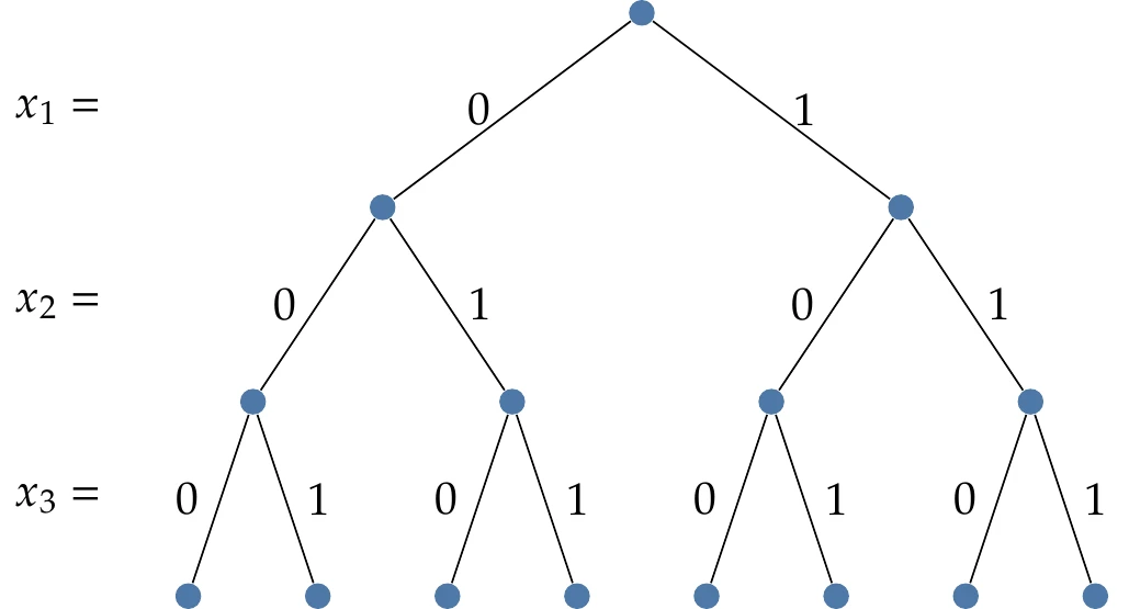
Figure 8.2:Enumerating the options for a binary problem with branching.

Figure 8.2 illustrates the branching concept for binary variables. If we explored all of those branches, this would amount to an exhaustive search. The main benefit of the branch-and-bound algorithm is that we can find ways to eliminate branches (referred to as pruning) to narrow down the search scope.

There are two ways to prune. If any of the relaxed problems is infeasible, we know that everything from that node downward (i.e., that branch) is also infeasible. Adding more constraints cannot make an infeasible problem feasible again. Thus, that branch is pruned, and we go back up the tree. We can also eliminate branches by determining that a better solution cannot exist on that branch. The algorithm keeps track of the best solution to the problem found so far.

If one of the relaxed problems returns an objective that is worse than the best we have found, we can prune that branch. We know this because adding constraints always leads to a solution that is either the same or worse, never better (assuming that we find the global optimum, which is guaranteed for LP problems).

The solution from a relaxed problem provides a lower bound—the best that could be achieved if continuing on that branch. The logic for these various possibilities is summarized in Algorithm 8.1.

The initial best known solution can be set as $f_\text{best} = \infty$ if nothing is known, but if a known feasible solution exists (or can be found quickly by some heuristic), providing any finite best point can speed up the optimization.

Many variations exist for the branch-and-bound algorithm. One variation arises from the choice of which variables to branch on at a given node.

One common strategy is to branch on the variable with the largest fractional component. For example, if $\hat{x} = [1.0, 0.4, 0.9, 0.0]$ , we could branch on $x_2$ or $x_3$ because both are fractional. We hypothesize that we are more likely to force the algorithm to make faster progress by branching on variables that are closer to midway between integers. In this case, that value would be $x_2 = 0.4$ . We would choose to branch on the value closest to 0.5, that is,

\min_i | x_i - 0.5 | \, .

(8.2)

Another variation of branch and bound arises from how the tree search is performed. Two common strategies are depth-first and breadth-first. A depth-first strategy continues as far down as possible (e.g., by always branching left) until it cannot go further, and then it follows right branches. A breadth-first strategy explores all nodes on a given level before increasing depth. Various other strategies exist. In general, we do not know beforehand which one is best for a given problem.

Depth-first is a common strategy because, in the absence of more information about a problem, it is most likely to be the fastest way to find a solution—reaching the bottom of the tree generally forces a solution. Finding a solution quickly is desirable because its solution can then be used as a lower bound on other branches.

The depth-first strategy requires less memory storage because breadth-first must maintain a longer history as the number of levels increases. In contrast, depth-first only requires node storage equal to the number of levels.

Algorithm 8.1 (Branch-and-bound algorithm)

Algorithm

\quad fbestf_\text{best}fbest​: Best known solution, if any; otherwise fbest=∞f_\text{best} = \inftyfbest​=∞
\quad x∗x^*x∗: Optimal point
\quad f(x∗)f(x^*)f(x∗): Optimal function value
Let S\mathcal{S}S be the set of indices for binary constrained design variables
while branches remain do
Solve relaxed problem for x^\hat xx^, f^\hat ff^​
if relaxed problem is infeasible then
Prune this branch, back up tree
if xi^∈{0,1} for all i∈S\hat{x_i} \in \{0, 1\} \text{ for all }  i \in \mathcal{S}xi​^​∈{0,1} for all i∈S then
A solution is foundfbestf_\text{best}fbest​ = min(fbest,f^f_\text{best}, \hat{f}fbest​,f^​), back up tree
if f^>fbest\hat f > f_\text{best}f^​>fbest​ then
Prune this branch, back up tree
A better solution might exist
Branch further

Example 8.4 (A binary branch-and-bound optimization)

Consider the following discrete problem with binary design variables:

\begin{aligned} \text{minimize} &\quad -2.5 x_1 -1.1 x_2 -0.9x_3 -1.5x_4\\ \text{subject to} &\quad 4.3x_1 + 3.8x_2 + 1.6x_3 + 2.1x_4 \le 9.2\\ &\quad 4 x_1 + 2 x_2 + 1.9 x_3 + 3 x_4 \le 9\\ &\quad x_i \in \{0, 1\} \text{ for all $i$} . \end{aligned}

To solve this problem, we begin at the first node by solving the linear relaxation. The binary constraint is removed and instead replaced with continuous bounds: $0 \le x_i \le 1$ . The solution to this LP is as follows:

\begin{aligned} x^* &= [1, 0.5274, 0.4975, 1]\\ f^* &= -5.0279. \end{aligned}

There are nonbinary values in the solution, so we need to branch. As mentioned previously, a typical choice is to branch on the variable with the most fractional component. In this case, that is $x_3$ , so we create two additional problems, which add the constraints $x_3 = 0$ and $x_3 = 1$ , respectively (Figure 8.3).

Figure 8.3:Initial binary branch.

Although depth-first was recommended previously, in this example, we use breadth-first because it yields a more concise example. The depth-first tree is also shown at the end of the example. We solve both of the problems at this next level as shown in Figure 8.4. Neither of these optimizations yields all binary values, so we have to branch both of them. In this case, the left node branches on $x_2$ (the only fractional component), and the right node also branches on $x_2$ (the most fractional component).

Figure 8.4:Solutions along these two branches.

The first branch (see Figure 8.5) yields a feasible binary solution! The corresponding function value $f = -4$ is saved as the best value so far. There is no need to continue on this branch because the solution cannot be improved on this particular branch.

Figure 8.5:The first feasible solution.

We continue solving along the rest of this row (Figure 8.6). The third node in this row yields another binary solution. In this case, the function value is $f = -4.9$ , which is better, so this becomes the new best value so far. The second and fourth nodes do not yield a solution. Typically, we would have to branch these further, but they have a lower bound that is worse than the best solution so far. Thus, we can prune both of these branches.

Figure 8.6:The rest of the solutions on this row.

All branches have been pruned, so we have solved the original problem:

\begin{aligned} x^* &= [1, 0, 1, 1] \\ f^* &= -4.9. \end{aligned}

Figure 8.7:Search path using a depth-first strategy.

Alternatively, we could have used a depth-first strategy. In this case, it is less efficient, but in general, the best strategy is not known beforehand. The depth-first tree for this same example is shown in Figure 8.7. Feasible solutions to the problem are shown as $f^*$ .

8.3.2 Integer Variables¶

If the problem cannot be cast in binary form, we can use the same procedure with integer variables. Instead of branching with two constraints ( $x_i = 0$ and $x_i = 1$ ), we branch with two inequality constraints that encourage integer solutions. For example, if the variable we branched on was $x_i = 3.4$ , we would branch with two new problems with the following constraints: $x_i \le 3$ or $x_i \ge 4$ .

Example 8.5 (Branch and bound with integer variables)

Consider the following problem:

\begin{aligned} \text{minimize} &\quad - x_1 -2 x_2 -3 x_3 -1.5 x_4\\ \text{subject to} &\quad x_1 + x_2 + 2x_3 + 2x_4 \le 10\\ &\quad 7 x_1 + 8 x_2 + 5 x_3 + x_4 = 31.5\\ &\quad x_i \in \mathbb{Z}^+ \text{ for } i = 1, 2, 3 \\ &\quad x_4 \ge 0 \, . \end{aligned}

We begin by solving the LP relaxation, replacing the integer constraints with a lower bound constraint of zero ( $x_i \ge 0$ ). The solution to that problem is

x^* = [0, 1.1818, 4.4091, 0], \quad f^* = -15.59 \, .

We begin by branching on the most fractional value, which is $x_3$ . We create two new branches:

The original LP with the added constraint $x_3 \le 4$
The original LP with the added constraint $x_3 \ge 5$

Even though depth-first is usually more efficient, we use breadth-first because it is easier to display on a figure. The solution to that first problem is

x^* = [0, 1.4, 4, 0.3], \quad f^* = -15.25.

The second problem is infeasible, so we can prune that branch.

Recall that the last variable is allowed to be continuous, so we now branch on $x_2$ by creating two new problems with additional constraints: $x_2 \le 1$ and $x_2 \ge 2$ .

The problem continues using the same procedure shown in the breadth-first tree in Figure 8.8. The figure gives some indication of why solving integer problems is more time-consuming than solving binary ones. Unlike the binary case, the same value is revisited with tighter constraints. For example, the constraint $x_3 \le 4$ is enforced early on. Later, two additional problems are created with tighter bounds on the same variable: $x_3 \le 2$ and $x_3 \ge 3$ . In general, the same variable could be revisited many times as the constraints are slowly tightened, whereas in the binary case, each variable is only visited once because the values can only be 0 or 1.

Figure 8.8:A breadth search of the mixed-integer programming example.

Once all the branches are pruned, we obtain the solution:

\begin{aligned} x^* &= [0, 2, 3, 0.5] \\ f^* &= -13.75. \end{aligned}

Nonconvex mixed-integer problems can also be used with the branch-and-bound method and generally use this latter strategy of forming two branches of continuous constraints. In this case, the relaxed problem is not a convex problem, so there is no guarantee that we have found a lower bound for that branch. Furthermore, the cost of each suboptimization problem is increased. Thus, for nonconvex discrete problems, this approach is usually only practical for a relatively small number of discrete design variables.

8.4 Greedy Algorithms¶

Greedy algorithms are among the simplest methods for discrete optimization problems. This method is more of a concept than a specific algorithm. The implementation varies with the application. The idea is to reduce the problem to a subset of smaller problems (often down to a single choice) and then make a locally optimal decision. That decision is locked in, and then the next small decision is made in the same manner. A greedy algorithm does not revisit past decisions and thus ignores much of the coupling between design variables.

Example 8.6 (A weighted directed graph)

As an example, consider the weighted directed graph shown in Figure 8.9. This graph might represent a transportation problem for shipping goods, information flow through a social network, or a supply chain problem. The objective is to traverse from node 1 to node 12 with the lowest possible total cost (the numbers above the path segments denote the cost of each path). A series of discrete choices must be made at each step, and those choices limit the available options in the next step.

Figure 8.9:The greedy algorithm in this weighted directed graph results in a total cost of 15, whereas the best possible cost is 10.

A greedy algorithm simply makes the best choice assuming each decision is the only decision to be made. Starting at node 1, we first choose to move to node 3 because that is the lowest cost between the three options (node 2 costs 2, node 3 costs 1, node 4 costs 5). We then choose to move to node 6 because that is the smallest cost between the next two available options (node 6 costs 4, node 7 costs 6), and so on. The path selected by the greedy algorithm is highlighted in the figure and results in a total cost of 15. The global optimum is also highlighted in the figure and has a total cost of 10.

The greedy algorithm used in Example 8.6 is easy to apply and scalable but does not generally find the global optimum. To find that global optimum, we have to consider the impact of our choices on future decisions. A method to achieve this for certain problem structures is discussed in the next section.

Even for a fixed problem, there are many ways to construct a greedy algorithm. The advantage of the greedy approach is that the algorithms are easy to construct, and they bound the computational expense of the problem. One disadvantage of the greedy approach is that it usually does not find an optimal solution (and in some cases finds the worst solution!1). Furthermore, the solution is not necessarily feasible. Despite the disadvantages, greedy algorithms can sometimes quickly find solutions reasonably close to an optimal solution.

Example 8.7 (Greedy algorithms)

A few other examples of greedy algorithms are listed below. For the traveling salesperson problem (Example 8.1), always select the nearest city as the next step. Consider the propeller problem (Example 8.2 but with additional discrete variables (number of blades, type of material, and number of shear webs). A greedy method could optimize the discrete variables one at a time, with the others fixed (i.e., optimize the number of blades first, fix that number, then optimize material, and so on). As a final example, consider the grocery store shopping problem discussed in a separate chapter (Example 11.1).^[3]A few possible greedy algorithms for this problem include: always pick the cheapest food item next, or always pick the most nutritious food item next, or always pick the food item with the most nutrition per unit cost.

8.5 Dynamic Programming¶

Dynamic programming is a valuable approach for discrete optimization problems with a particular structure. This structure can also be exploited in continuous optimization problems and problems beyond optimization. The required structure is that the problem can be posed as a Markov chain (for continuous problems, this is called a Markov process). A Markov chain or process satisfies the Markov property, where a future state can be predicted from the current state without needing to know the entire history. The concept can be generalized to a finite number of states (i.e., more than one but not the entire history) and is called a variable-order Markov chain.

If the Markov property holds, we can transform the problem into a recursive one. Using recursion, a smaller problem is solved first, and then larger problems are solved that use the solutions from the smaller problems.

This approach may sound like a greedy optimization, but it is not. We are not using a heuristic but fully solving the smaller problems. Because of the problem structure, we can reuse those solutions. We will illustrate this in examples. This approach has become particularly useful in optimal control and some areas of economics and computational biology. More general design problems, such as the propeller example (Example 8.2), do not fit this type of structure (i.e., choosing the number of blades cannot be broken up into a smaller problem separate from choosing the material).

A classic example of a Markov chain is the Fibonacci sequence, defined as follows:

\begin{aligned} f_0 &= 0\\ f_1 &= 1\\ f_n &= f_{n-1} + f_{n-2} . \end{aligned}

(8.3)

We can compute the next number in the sequence using only the last two states.^[4]We could implement the computation of this sequence using recursion, as shown algorithmically in Algorithm 8.2 and graphically in Figure 8.10 for $f_5$ .

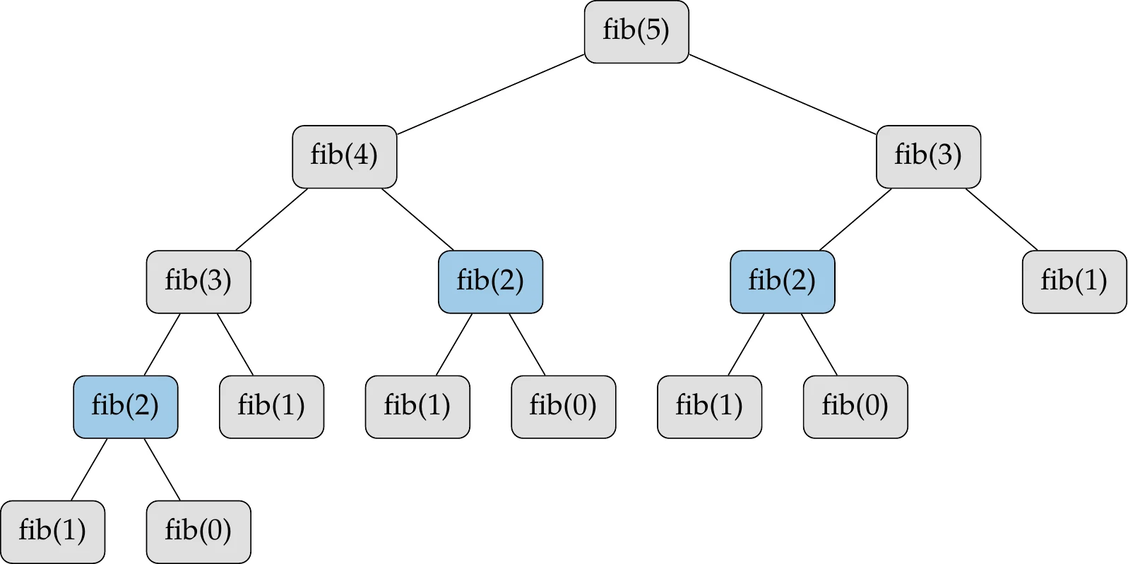
Computing Fibonacci sequence using recursion. The function fib(2) is highlighted as an example to show the repetition that occurs in this recursive procedure. — Figure 8.10:Computing Fibonacci sequence using recursion. The function `fib(2)` is highlighted as an example to show the repetition that occurs in this recursive procedure.

Although this recursive procedure is simple, it is inefficient. For example, the calculation for fib(2) (highlighted in Figure 8.10) is repeated multiple times. There are two main approaches to avoiding this inefficiency. The first is a top-down procedure called memoization, where we store previously computed values to avoid having to compute them again. For example, the first time we need fib(2), we call the fib function and store the result (the value 1). As we progress down the tree, if we need fib(2) again, we do not call the function but retrieve the stored value instead.

A bottom-up procedure called tabulation is more common. This procedure is how we would typically show the Fibonacci sequence. We start from the bottom ( $f_0$ ) and work our way forward, computing each new value using the previous states. Rather than using recursion, this involves a simple loop, as shown in Algorithm 8.3. Whereas memoization fills entries on demand, tabulation systematically works its way up, filling in entries. In either case, we reduce the computational complexity of this algorithm from exponential complexity (approximately $\mathcal{O}(2^n)$ ) to linear complexity ( $\mathcal{O}(n)$ ).

These procedures can be applied to optimization, but before introducing examples, we formalize the mathematics of the approach. One main difference in optimization is that we do not have a set formula like a Fibonacci sequence. Instead, we need to make a design decision at each state, which changes the next state. For example, in the problem shown in Figure 8.9, we decide which path to take.

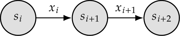
Figure 8.11:Diagram of state transitions in a Markov chain.

Mathematically, we express a given state as $s_i$ and make a design decision $x_i$ , which transitions us to the next state $s_{i+1}$ (Figure 8.11),

s_{i+1} = t_i(s_i, x_i),

(8.4)

where $t$ is a transition function.^[5]At each transition, we compute the cost function $c$ .^[6]For generality, we specify a cost function that may change at each iteration $i$ :

c_i(s_i, x_i) .

(8.5)

We want to make a set of decisions that minimize the sum of the current and future costs up to a certain time, which is called the value function,

v(s_i) = \underset{x_i, \ldots, x_n}{\text{minimize}}\; \left( c_i(s_i, x_i) + c_{i+1}(s_{i+1}, x_{i+1}) + \ldots + c_n(s_n, x_n) \right) ,

(8.6)

where $n$ defines the time horizon up to which we consider the cost. For continuous problems, the time horizon may be infinite. The value function (Equation 8.6) is the minimum cost, not just the cost for some arbitrary set of decisions.^[7]Bellman’s principle of optimality states that because of the structure of the problem (where the next state only depends on the current state), we can determine the best solution at this iteration $x_i^*$ if we already know all the optimal future decisions $x_{i+1}^*, \ldots, x_{n}^*$ . Thus, we can recursively solve this problem from the back (bottom) by determining $x_n^*$ , then $x_{n-1}^*$ , and so on back to $x_i^*$ . Mathematically, this recursive procedure is captured by the Bellman equation:

v(s_i) = \underset{x_i}{\text{minimize}} \left( c(s_i, x_i) + v(s_{i+1}) \right) \, .

(8.7)

We can also express this equation in terms of our transition function to show the dependence on the current decision:

v(s_i) = \underset{x_i}{\text{minimize}} \left( c(s_i, x_i) + v(t_i(s_i, x_i)) \right) \, .

(8.8)

Example 8.8 (Dynamic programming applied to a graph problem)

Let us solve the graph problem posed in Example 8.6 using dynamic programming. For convenience, we repeat a smaller version of the figure in Figure 8.12. We use the tabulation (bottom-up) approach. To do this, we construct a table where we keep track of the cost to move from this node to the end (node 12) and which node we should move to next:

Node	1	2	3	4	5	6	7	8	9	10	11	12
Cost
Next

Figure 8.12:Small version of Figure 8.9 for convenience.

We start from the end. The last node is simple: there is no cost to move from node 12 to the end (we are already there), and there is no next node.

Node	1	2	3	4	5	6	7	8	9	10	11	12
Cost												0
Next												–

Now we move back one level to consider nodes 9, 10, and 11. These nodes all lead to node 12 and are thus straightforward. We need to be more careful with the formulas as we get to the more complicated cases next.

Node	1	2	3	4	5	6	7	8	9	10	11	12
Cost									3	6	2	0
Next									12	12	12	–

Now we move back one level to nodes 5, 6, 7, and 8. Using the Bellman equation for node 5, the cost is

\text{cost}(5) = \min[3 + \text{cost}(9), 2 + \text{cost}(10), 1 + \text{cost}(11)].

(8.9)

We have already computed the minimum value for cost(9), cost(10), and cost(11), so we just look up these values in the table. In this case, the minimum total value is 3 and is associated with moving to node 11. Similarly, the cost for node 6 is

\text{cost}(6) = \min[5 + \text{cost}(9), 4 + \text{cost}(10)] .

(8.10)

The result is 8, and it is realized by moving to node 9.

Node	1	2	3	4	5	6	7	8	9	10	11	12
Cost					3	8			3	6	2	0
Next					11	9			12	12	12	–

We repeat this process, moving back and reusing optimal solutions to find the global optimum. The completed table is as follows:

Node	1	2	3	4	5	6	7	8	9	10	11	12
Cost	10	8	12	9	3	8	7	4	3	6	2	0
Next	2	5	6	8	11	9	11	11	12	12	12	–

From this table, we see that the minimum cost is 10. This cost is achieved by moving first to node 2. Under node 2, we see that we next go to node 5, then 11, and finally 12. Thus, the tabulation gives us the global minimum for cost and the design decisions to achieve that.

To illustrate the concepts more generally, consider another classic problem in discrete optimization—the knapsack problem. In this problem, we have a fixed set of items we can select from. Each item has a weight $w_i$ and a cost $c_i$ . Because the knapsack problem is usually written as a maximization problem and cost implies minimization, we should use value instead. However, we proceed with cost to be consistent with our earlier notation. The knapsack has a fixed capacity $K$ (a scalar) that cannot be exceeded.

The objective is to choose the items that yield the highest total cost subject to the capacity of our knapsack. The design variables $x_i$ are either 1 or 0, indicating whether we take or do not take item $i$ . This problem has many practical applications, such as shipping, data transfer, and investment portfolio selection.

The problem can be written as

\begin{aligned} \underset{x}{\text{maximize}} &\quad \sum_{i=1}^n c_i x_i \\ \text{subject to} &\quad \sum_{i=1}^n w_i x_i \le K\\ &\quad x_i \in \{0, 1\} \,. \end{aligned}

(8.11)

In its present form, the knapsack problem has a linear objective and linear constraints, so branch and bound would be a good approach. However, this problem can also be formulated as a Markov chain, so we can use dynamic programming. The dynamic programming version accommodates variations such as stochasticity and other constraints more easily.

To pose this problem as a Markov chain, we define the state as the remaining capacity of the knapsack $k$ and the number of items we have already considered. In other words, we are interested in $v(k, i)$ , where $v$ is the value function (optimal value given the inputs), $k$ is the remaining capacity in the knapsack, and $i$ indicates that we have already considered items 1 through $i$ (this does not mean we have added them all to our knapsack, only that we have considered them). We iterate through a series of decisions $x_i$ deciding whether to take item $i$ or not, which transitions us to a new state where $i$ increases and $k$ may decrease, depending on whether or not we took the item.

The real problem we are interested in is $v(K, n)$ , which we solve using tabulation. Starting at the bottom, we know that $v(k, 0) = 0$ for any $k$ . This means that no matter the capacity, the value is 0 if we have not considered any items yet. To work forward, consider a general case considering item $i$ , with the assumption that we have already solved up to item $i-1$ for any capacity. If item $i$ cannot fit in our knapsack ( $w_i > k$ ), then we cannot take the item. Alternatively, if the weight is less than the capacity, we need to decide whether to select item $i$ or not. If we do not, then the value is unchanged, and $v(k, i) = v(k, i-1)$ . If we do select item $i$ , then our value is $c_i$ plus the best we could do with the previous items but with a capacity that was smaller by $w_i$ : $v(k, i) = c_i + v(k-w_i, i-1)$ . Whichever of these decisions yields a better value is what we should choose.

To determine which items produce this cost, we need to add more logic. To keep track of the selected items, we define a selection matrix $S$ of the same size as $v$ (note that this matrix is indexed starting at zero in both dimensions). Every time we accept an item $i$ , we register that in the matrix as $S_{k,i} = 1$ . Algorithm 8.4 summarizes this process.

Algorithm 8.4 (Knapsack with tabulation)

Algorithm

\quad cic_ici​: Cost of item iii
\quad wiw_iwi​: Weight of item iii
\quad KKK: Total available capacity
\quad x∗x^*x∗: Optimal selections
\quad v(K,n)v(K, n)v(K,n): Corresponding cost, v(k,i)v(k, i)v(k,i) is the optimal cost for capacity kkk considering items 1 through iii; note that indexing starts at 0
for k=0k = 0k=0 to  KKK do
v(k,0)=0v(k, 0) = 0v(k,0)=0 No items considered; value is zero for any capacity
for i=1i = 1i=1 to  nnn do
Iterate forward solving for one additional item at a timefor k=0k = 0k=0 to  KKK do
if wi>kw_i > kwi​>k then
v(k,i)=v(k,i−1)v(k, i) = v(k, i-1)v(k,i)=v(k,i−1) Weight exceeds capacity; value unchanged
if ci+v(k−wi,i−1)>v(k,i−1)c_i + v(k-w_i, i-1) > v(k, i-1)ci​+v(k−wi​,i−1)>v(k,i−1) then
Take itemv(k,i)=ci+v(k−wi,i−1)v(k, i) = c_i + v(k-w_i, i-1)v(k,i)=ci​+v(k−wi​,i−1)
S(k,i)=1S(k, i) = 1S(k,i)=1
Reject item
v(k,i)=v(k,i−1)v(k, i) = v(k, i-1)v(k,i)=v(k,i−1)
k=Kk = Kk=K Initialize
x∗={}x^* = \{\}x∗={} Initialize solution x∗x^*x∗ as an empty set
for i=ni = ni=n to  1 by  -1 do
Loop to determine which items we selectedif Sk,i=1S_{k,i} = 1Sk,i​=1 then
add iii to x∗x^*x∗ Item iii was selected
k=k−wik = k - w_ik=k−wi​

We fill all entries in the matrix $v[k, i]$ to extract the last value $v[K, n]$ . For small numbers, filling this matrix (or table) is often illustrated manually, hence the name tabulation. As with the Fibonacci example, using dynamic programming instead of a fully recursive solution reduces the complexity from $\mathcal{O}(2^n)$ to $\mathcal{O}(Kn)$ , which means it is pseudolinear. It is only pseudolinear because there is a dependence on the knapsack size. For small capacities, the problem scales well even with many items, but as the capacity grows, the problem scales much less efficiently. Note that the knapsack problem requires integer weights. Real numbers can be scaled up to integers (e.g., 1.2, 2.4 become 12, 24). Arbitrary precision floats are not feasible given the number of combinations to search across.

Example 8.9 (Knapsack problem with dynamic programming)

Consider five items with the following weights and costs:

\begin{aligned} w_i &= [4, 5, 2, 6, 1]\\ c_i &= [4, 3, 3, 7, 2]. \end{aligned}

The capacity of our knapsack is $K = 10$ . Using Algorithm 8.4, we find that the optimal cost is 12. The value matrix is as follows:

\begin{bmatrix} 0 & 0 & 0 & 0 & 0 & 0\\ 0 & 0 & 0 & 0 & 0 & 2\\ 0 & 0 & 0 & 3 & 3 & 3\\ 0 & 0 & 0 & 3 & 3 & 5\\ 0 & 4 & 4 & 4 & 4 & 5\\ 0 & 4 & 4 & 4 & 4 & 6\\ 0 & 4 & 4 & 7 & 7 & 7\\ 0 & 4 & 4 & 7 & 7 & 9\\ 0 & 4 & 4 & 7 & 10 & 10\\ 0 & 4 & 7 & 7 & 10 & 12\\ 0 & 4 & 7 & 7 & 11 & 12 \end{bmatrix}.

For this example, the selection matrix $S$ is as follows:

S = \begin{bmatrix} 0 & 0 & 0 & 0 & 0 & 0\\ 0 & 0 & 0 & 0 & 0 & 1\\ 0 & 0 & 0 & 1 & 0 & 0\\ 0 & 0 & 0 & 1 & 0 & 1\\ 0 & 1 & 0 & 0 & 0 & 1\\ 0 & 1 & 0 & 0 & 0 & 1\\ 0 & 1 & 0 & 1 & 0 & 0\\ 0 & 1 & 0 & 1 & 0 & 1\\ 0 & 1 & 0 & 1 & 1 & 0\\ 0 & 1 & 1 & 0 & 1 & 1\\ 0 & 1 & 1 & 0 & 1 & 1 \end{bmatrix}.

Following this algorithm, we find that we selected items 3, 4, and 5 for a total cost of 12, as expected, and a total weight of 9.

Like greedy algorithms, dynamic programming is more of a technique than a specific algorithm. The implementation varies with the particular application.

8.6 Simulated Annealing¶

Simulated annealing^[8]is a methodology designed for discrete optimization problems. However, it can also be effective for continuous multimodal problems, as we will discuss.

The algorithm is inspired by the annealing process of metals. The atoms in a metal form a crystal lattice structure. If the metal is heated, the atoms move around freely. As the metal cools down, the atoms slow down, and if the cooling is slow enough, they reconfigure into a minimum-energy state. Alternatively, if the metal is quenched or cooled rapidly, the metal recrystallizes with a different higher-energy state (called an amorphous metal).

From statistical mechanics, the Boltzmann distribution (also called Gibbs distribution) describes the probability of a system occupying a given energy state:

P(e) \propto \exp\left(\frac{-e}{k_B T}\right) \, ,

(8.12)

where $e$ is the energy level, $T$ is the temperature, and $k_B$ is Boltzmann’s constant. This equation shows that as the temperature decreases, the probability of occupying a higher-energy state decreases, but it is not zero. Therefore, unlike in classical mechanics, an atom could jump to a higher-energy state with some small probability. This property imparts an exploratory nature to the optimization algorithm, which avoids premature convergence to a local minimum. The temperature level provides some control on the level of expected exploration.

An early approach to simulate this type of probabilistic thermodynamic model was the Metropolis algorithm.4 In the Metropolis algorithm, the probability of transitioning from energy state $e_1$ to energy state $e_2$ is formulated as

P = \min\left(\exp\left(\frac{-(e_2 - e_1)}{k_B T}\right), 1 \right) \, ,

(8.13)

where this probability is limited to be no greater than 1. This limit is needed because the exponent yields a value greater than 1 when $e_2 < e_1$ , which would be nonsensical. Simulated annealing leverages this concept in creating an optimization algorithm.

In the optimization analogy, the objective function is the energy level. Temperature is a parameter controlled by the optimizer, which begins high and is slowly “cooled” to drive convergence. At a given iteration, the design variables are given by $x$ , and the objective (or energy) is given by $f(x^{(k)})$ . A new state $x_{\text{new}}$ is selected at random in the neighborhood of $x$ . If the energy level decreases, the new state is accepted. If the energy level increases, the new state might still be accepted with probability

\exp\left(\frac{-\left(f(x_{\text{new}}) - f\left(x^{(k)}\right)\right)}{T}\right) ,

(8.14)

where Boltzmann’s constant is removed because it is just an arbitrary scale factor in the optimization context. Otherwise, the state remains unchanged. Constraints can be handled in this algorithm without resorting to penalties by rejecting any infeasible step.

We must supply the optimizer with a function that provides a random neighboring design from the set of possible design configurations. A neighboring design is usually related to the current design instead of picking a pure random design from the entire set. In defining the neighborhood structure, we might wish to define transition probabilities so that all neighbors are not equally likely. This type of structure is common in Markov chain problems. Because the nature of different discrete problems varies widely, we cannot provide a generic neighbor-selecting algorithm, but an example is shown later for the specific case of a traveling salesperson problem.

Finally, we need to determine the annealing schedule (or cooling schedule), a process for decreasing the temperature throughout the optimization. A common approach is an exponential decrease:

T = T_0 \alpha^k \, ,

(8.15)

where $T_0$ is the initial temperature, $\alpha$ is the cooling rate, and $k$ is the iteration number. The cooling rate $\alpha$ is a number close to 1, such as 0.8–0.99. Another simple approach to iterate toward zero temperature is as follows:

T = T_0 \left(1 - \frac{k}{k_{\max}} \right)^\beta \, ,

(8.16)

where the exponent $\beta$ is usually in the range of 1–4. A higher exponent corresponds to spending more time at low temperatures. In many approaches, the temperature is kept constant for a fixed number of iterations (or a fixed number of successful moves) before moving to the next decrease. Many methods are simple schedules with a predetermined rate, although more complex adaptive methods also exist.^[9] The annealing schedule can substantially impact the algorithm’s performance, and some experimentation is required to select an appropriate schedule for the problem at hand. One essential requirement is that the temperature should start high enough to allow for exploration. This should be significantly higher than the maximum expected energy change (change in objective) but not so high that computational time is wasted with too much random searching. Also, cooling should occur slowly to improve the ability to recover from a local optimum, imitating the annealing process instead of the quenching process.

The algorithm is summarized in Algorithm 8.5; for simplicity in the description, the annealing schedule uses an exponential decrease at every iteration.

Algorithm 8.5 (Simulated Annealing)

Algorithm

Inputs:

$\quad$ $x_{0}$ : Starting point

$\quad$ $T_{0}$ : Initial temperature

Outputs:

$\quad$ $x^*$ : Optimal point

for $k = 0$ to $k_{\max}$ do

Simple iteration; convergence metrics can be used instead

$x_{\text{new}}$ = neighbor $\left(x^{(k)}\right)$ Randomly generate from neighbors

if $f(x_{\text{new}}) \le f\left(x^{(k)}\right)$ then

Energy decreased; jump to new state

$x^{(k+1)} = x_{\text{new}}$

else

$r \in \mathcal{U}[0, 1]$ Randomly draw from uniform distribution

$P = \exp\left(\frac{-\left(f(x_{\text{new}}) - f\left(x^{(k)}\right)\right)}{T}\right)$

if $P \ge r$ then

Probability high enough to jump

$x^{(k+1)} = x_{\text{new}}$

else

$x^{(k+1)} = x^{(k)}$ Otherwise remain at current state

end if

$T = \alpha T$ Reduce temperature

end for

Example 8.10 (Traveling salesperson with simulated annealing)

This example sets up the traveling salesperson problem with 50 points randomly distributed (from uniform sampling) on a square grid with sides of length 1 (left of Figure 8.13). The objective is the total Euclidean distance of a path that traverses all points and returns to the starting point. The design variables are a sequence of integers corresponding to the order in which the salesperson traverses the points.

We generate new neighboring designs using the technique from Lin,6 where one of two options is randomly chosen at each iteration: (1) randomly choose two points and flip the direction of the path segments between those two points, or (2) randomly choose two points and move the path segments to follow another randomly chosen point. The distance traveled by the randomly generated initial set of points is 26.2.

We specify an iteration budget of 25,000 iterations, set the initial temperature to be 10, and decrease the temperature by a multiplicative factor of 0.95 at every 100 iterations. The right panel of Figure 8.13 shows the final path, which has a length of 5.61. The final path might not be the global optimum (remember, these finite time methods are only approximations of the full combinatorial search), but the methodology is effective and fast for this problem in finding at least a near-optimal solution. Figure 8.14 shows the iteration history.

Figure 8.13:Initial and final paths for traveling salesperson problem.

Figure 8.14:Convergence history of the simulated annealing algorithm.

The simulated annealing algorithm can be applied to continuous multimodal problems as well. The motivation is similar because the initial high temperature permits the optimizer to escape local minima, whereas a purely descent-based approach would not. By slowly cooling, the initial exploration gives way to exploitation. The only real change in the procedure is in the neighbor function. A typical approach is to generate a random direction and choose a step size proportional to the temperature. Thus, smaller, more conservative steps are taken as the algorithm progresses. If bound constraints are present, they would be enforced at this step. Purely random step directions are not particularly efficient for many continuous problems, particularly when most directions are ill-conditioned (e.g., a narrow valley or near convergence). One variation adopts concepts from the Nelder–Mead algorithm (Section 7.3) to improve efficiency.7 Overall, simulated annealing has made more impact on discrete problems compared with continuous ones.

8.7 Binary Genetic Algorithms¶

The binary form of a genetic algorithm (GA) can be directly used with discrete variables. Because the binary form already requires a discrete representation for the population members, using discrete design variables is a natural fit. The details of this method were discussed in Section 7.6.1.

8.8 Summary¶

This chapter discussed various strategies for approaching discrete optimization problems. Some problems can be well approximated using rounding, can be reparameterized in a continuous way, or only have a few discrete combinations, allowing for explicit enumeration. For problems that can be posed as linear (or convex in general), branch and bound is effective. If the problem can be posed as a Markov chain, dynamic programming is a useful method.

If none of these categorizations are applicable, then a stochastic method, such as simulated annealing or GAs, may work well. These stochastic methods typically struggle as the dimensionality of the problem increases. However, simulated annealing can scale better for some problems if there are clever ways to quickly evaluate designs in the neighborhood, as is done with the traveling salesperson problem. An alternative to these various algorithms is to use a greedy strategy, which can scale well. Because this strategy is a heuristic, it usually results in a loss in solution quality.

Problems¶

Exercise 1

Answer true or false and justify your answer.

All discrete variables can be represented by integers.
Discrete optimization algorithms sometimes use heuristics and find only approximate solutions.
The rounding technique solves a discrete optimization problem with continuous variables and then rounds each resulting design variable, objective, and constraint to the nearest integer.
Exhaustive search is the only way to be sure we have found the global minimum for a problem that involves discrete variables.
The branch-and-bound method is guaranteed to find the global optimum for convex problems.
When using the branch-and-bound method for binary variables, the same variable might have to be revisited.
When using the branch-and-bound method, the breadth-first strategy requires less memory storage than the depth-first strategy.
Greedy algorithms never reconsider a decision once it has been made.
The Markov property applies when a future state can be predicted from the current state without needing to know any previous state.
Both memoization and tabulation reduce the computational complexity of dynamic programming such that it no longer scales exponentially.
Simulated annealing can be used to minimize smooth unimodal functions of continuous design variables.
Simulated annealing, genetic algorithms, and dynamic programming include stochastic procedures.

Exercise 2

Branch and bound. Solve the following problem using a manual branch-and-bound approach (i.e., show each LP subproblem), as is done in Example 8.4:

\begin{aligned} \text{maximize} &\quad 0.5 x_1 + 2 x_2 + 3.5 x_3 + 4.5 x_4\\ \text{subject to} &\quad 5.5 x_1 + 0.5 x_2 + 3.5 x_3 + 2.3 x_4 \le 9.2\\ &\quad 2 x_1 + 4 x_2 + 2 x_4 \le 8\\ &\quad 1 x_1 + 3 x_2 + 3 x_3 + 4 x_4 \le 4\\ &\quad x_i \in \{0, 1\} \text{ for all $i$}. \end{aligned}

Exercise 3

Solve an integer linear programming problem. A chemical company produces four types of products: A, B, C, and D. Each requires labor to produce and uses some combination of chlorine, sulfuric acid, and sodium hydroxide in the process. The production process can also produce these chemicals as a by-product, rather than just consuming them. The chemical mixture and labor required for the production of the three products are listed in the following table, along with the availability per day. The market values for one barrel of A, B, C, and D are $50, $30, $80, and $30, respectively. Determine the number of barrels of each to produce to maximize profit using three different approaches:

As a continuous linear programming problem with rounding
As an integer linear programming problem
Exhaustive search

	A	B	C	D	Limit
Chlorine	0.74	$-$ 0.05	1.0	$-$ 0.15	97
Sodium hydroxide	0.39	0.4	0.91	0.44	99
Sulfuric acid	0.86	0.89	0.09	0.83	52
Labor (person-hours)	5	7	7	6	1000

Discuss the results.

Footnotes¶

Sometimes subtle differences in meaning are intended, but typically, and in this chapter, these terms can be used interchangeably.
↩
Better methods may exist that leverage the specific problem structure, some of which are discussed in this chapter.
↩
This is a form of the knapsack problem, which is a classic problem in discrete optimization discussed in more detail in the following section.
↩
We can also convert this to a standard first-order Markov chain by defining $g_n = f_{n-1}$ and considering our state to be $(f_n, g_n)$ . Then, each state only depends on the previous state.
↩
For some problems, the transition function is stochastic.
↩
It is common to use discount factors on future costs.
↩
We use $v$ and $c$ for the scalars in Equation 8.6 instead of Greek letters because the connection to “value” and “cost” is clearer.
↩
First developed by 2 and 3
↩
See 5, for example.
↩

References¶

Gutin, G., Yeo, A., & Zverovich, A. (2002). Traveling salesman should not be greedy: domination analysis of greedy-type heuristics for the TSP. Discrete Applied Mathematics, 117(1–3), 81–86. 10.1016/s0166-218x(01)00195-0
Kirkpatrick, S., Gelatt, C. D., & Vecchi, M. P. (1983). Optimization by simulated annealing. Science, 220(4598), 671–680. 10.1126/science.220.4598.671
Černý, V. (1985). Thermodynamical approach to the traveling salesman problem: An efficient simulation algorithm. Journal of Optimization Theory and Applications, 45(1), 41–51. 10.1007/bf00940812
Metropolis, N., Rosenbluth, A. W., Rosenbluth, M. N., Teller, A. H., & Teller, E. (1953). Equation of state calculations by fast computing machines. Journal of Chemical Physics. 10.2172/4390578
Andresen, B., & Gordon, J. M. (1994). Constant thermodynamic speed for minimizing entropy production in thermodynamic processes and simulated annealing. Physical Review E, 50(6), 4346–4351. 10.1103/physreve.50.4346
Lin, S. (1965). Computer solutions of the traveling salesman problem. Bell System Technical Journal, 44(10), 2245–2269. 10.1002/j.1538-7305.1965.tb04146.x
Press, W. H., Wevers, J. C. A., Flannery, B. P. ., Teukolsky, S. A., Vetterling, W. T., Flannery, B. P., & Vetterling, W. T. . (1992). Numerical Recipes in C: The Art of Scientific Computing. Cambridge University Press.

8 Discrete Optimization

8.1 Binary, Integer, and Discrete Variables¶

8.2 Avoiding Discrete Variables¶

8.3 Branch and Bound¶

8.3.1 Binary Variables¶

8.3.2 Integer Variables¶

8.4 Greedy Algorithms¶

8.5 Dynamic Programming¶

8.6 Simulated Annealing¶

8.7 Binary Genetic Algorithms¶

8.8 Summary¶

Problems¶