12 Optimization Under Uncertainty
Uncertainty is always present in engineering design. Manufacturing processes create deviations from the specifications, operating conditions vary from the ideal, and some parameters are inherently variable. Optimization with deterministic inputs can lead to poorly performing designs. Optimization under uncertainty (OUU) is the optimization of systems in the presence of random parameters or design variables. The objective is to produce robust and reliable designs. A design is robust when the objective function is less sensitive to inherent variability. A design is reliable when it is less prone to violating a constraint when accounting for the variability.[1]This chapter discusses how uncertainty can be used in the objective function to obtain robust designs and how it can be used in constraints to get reliable designs. We introduce methods that propagate input uncertainties through a computational model to produce output statistics.
We assume familiarity with basic statistics concepts such as expected value, variance, probability density functions (PDFs), cumulative distribution functions (CDFs), and some common probability distributions. A brief review of these topics is provided in Section A.9 if needed.
12.1 Robust Design
We call a design robust if its performance is less sensitive to inherent variability. In optimization, “performance” is directly associated with the objective function. Satisfying the design constraints is a requirement, but adding a margin to a constraint does not increase performance in the standard optimization formulation. Thus, for a robust design, the objective function is less sensitive to variations in the random design variables and parameters. We can achieve this by formulating an objective function that considers such variations and reflects uncertainty.
A common example of robust design is considering the performance of an engineering device at different operating conditions. If we had deterministic operating conditions, it would make sense to maximize the performance for those conditions. For example, suppose we knew the exact wind speeds and wind directions a sailboat would experience in a race. In that case, we could optimize the hull and sail design to minimize the time around the course. Unfortunately, if variability does exist, the sailboat designed for deterministic conditions will likely perform poorly in off-design conditions. A better strategy considers the uncertainty in the operating conditions and maximizes the expected performance across a range of conditions. A robust design achieves good performance even with uncertain wind speeds and directions.
There are many options for formulating robust design optimization problems. The most common OUU objective is to minimize the expected value of the objective function . This yields robust designs because the average performance under variability is considered.
Consider the function shown on the left in Figure 12.1. If is deterministic, minimizing this function yields the global minimum on the right. Now consider what happens when is uncertain. “Uncertain” means that is no longer a deterministic input. Instead, it is a random variable with some probability distribution. For example, represents a random variable with a mean of . We can compute the average value of the objective at each from the expected value of a function (Equation A.65):
and is a dummy variable for integration. Repeating this integral at each value gives the expected value as a function of .
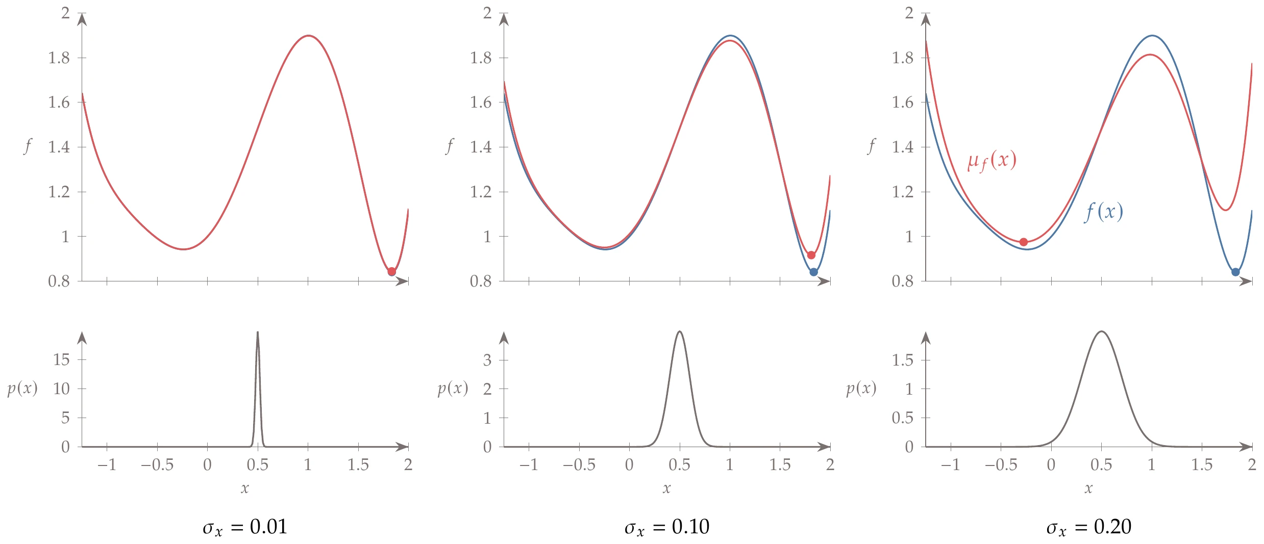
Figure 12.1:The global minimum of the expected value can shift depending on the standard deviation of , . The bottom row of figures shows the normal probability distributions at .
Figure 12.1 shows the expected value of the objective for three different standard deviations. The probability distribution of for a mean value of and three different standard deviations is shown on the bottom row the figure. For a small variance (), the expected value function is indistinguishable from the deterministic function , and the global minimum is the same for both functions. However, for , the minimum of the expected value function is different from that of the deterministic function. Therefore, the minimum on the right is not as robust as the one on the left. The minimum one on the right is a narrow valley, so the expected value increases rapidly with increased variance. The opposite is true for the minimum on the left. Because it is in a broad valley, the expected value is less sensitive to variability in . Thus, a design whose performance changes rapidly with respect to variability is not robust.
Of course, the mean is just one possible statistical output metric. Variance, or standard deviation (), is another common metric. However, directly minimizing the variance is less common because although low variability is often desirable, such an objective has no incentive to improve mean performance and so usually performs poorly. These two metrics represent a trade-off between risk (variance) and reward (mean). The compromise between these two metrics can be quantified through multiobjective optimization (see Chapter 9), which would result in a Pareto front with the notional behavior illustrated in Figure 12.2.
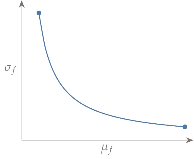
Figure 12.2:When designing for robustness, there is an inherent trade-off between risk (represented by the variance, ) and reward (represented by the expected value, ).
Because both multiobjective optimization and uncertainty quantification are costly, the overall cost of producing such a Pareto front might be prohibitive. Therefore, we might instead seek to minimize the expected value while constraining the variance to a value that the designer can tolerate. Another option is to minimize the mean plus weighted standard deviations.
Many other relevant statistical objectives do not involve statistical moments like mean or variance. Examples include minimizing the 95th percentile of the distribution or employing a reliability metric, , that minimizes the probability that the objective exceeds some critical value.
12.2 Reliable Design
We call a design reliable when it is less prone to failure under variability. In other words, the constraints have a lower probability of being violated under variations in the random design variables and parameters. In a robust design, we consider the effect of uncertainty on the objective function. In reliable design, we consider that effect on the constraints.
A common example of reliability is structural safety. Consider Example 3.9, where we formulated a mass minimization subject to stress constraints. In such structural optimization problems, many of the stress constraints are active at the optimum. Constraining the stress to be equal to or below the yield stress value as if this value were deterministic is probably not a good idea because variations in the material properties or manufacturing could result in structural failure. Instead, we might want to include this variability so that we can reduce the probability of failure.
To generate a reliable design, we want the probability of satisfying the constraints to exceed some preselected reliability level. Thus, we change deterministic inequality constraints to ensure that the probability of constraint satisfaction exceeds a specified reliability level , that is,
For example, if we set , then constraint must be satisfied with a probability of 99.9 percent. Thus, we can explicitly set the reliability level that we wish to achieve, with associated trade-offs in the level of performance for the objective function.
In some engineering disciplines, increasing reliability is handled simply through safety factors. These safety factors are deterministic but are usually derived through statistical means.
12.3 Forward Propagation
In the previous sections, we have assumed that we know the statistics (e.g., mean and standard deviation) of the outputs of interest (objectives and constraints). However, we generally do not have that information. Instead, we might only know the PDFs of the inputs.[5]Forward-propagation methods propagate input uncertainties through a numerical model to compute output statistics.
Uncertainty quantification is a large field unto itself, and we only provide an introduction to it in this chapter. We introduce four well-known nonintrusive methods for forward propagation: first-order perturbation methods, direct quadrature, Monte Carlo methods, and polynomial chaos.
12.3.1 First-Order Perturbation Method
Perturbation methods are based on a local Taylor series expansion of the functional output. In the following, represents an output of interest, and represents all the random variables (not necessarily all the variables that depends on). A first-order Taylor series approximation of about the mean of is given by
where is the dimensionality of . We can estimate the average value of by taking the expected value of both sides and using the linearity of expectation as follows:
The last first-order term is zero, so we can write
That is, when considering only first-order terms, the mean of the function is the function evaluated at the mean of the input.
The variance of is given by
The expectation term in this equation is the covariance matrix , so we can write this in matrix notation as
We often assume that each random input variable is mutually independent. This is true for the design variables for a well-posed optimization problem, but the parameters may or may not be independent.
When the parameters are independent (this assumption is often made even if not strictly true), the covariance matrix is diagonal, and the variance estimation simplifies to
These equations are frequently used to propagate errors from experimental measurements. Major limitations of this approach are that (1) it relies on a linearization (first-order Taylor series), which has limited accuracy;[6](2) it assumes that all uncertain parameters are uncorrelated, which is true for design variables but is not necessarily true for parameters (this assumption can be relaxed by providing the covariances); and (3) it implicitly assumes symmetry in the input distributions because we neglect all higher-order moments (e.g., skewness, kurtosis) and is, therefore, less applicable for problems that are highly asymmetric, such as the wind farm example (Example 12.2).
We have not assumed that the input or output distributions are normal probability distributions (i.e., Gaussian). However, we can only estimate the mean and variance with a first-order series and not the higher-order moments.
The equation for the variance (Equation 12.8) is straightforward, but the derivative terms can be challenging when using gradient-based optimization.
The first-order derivatives in Equation 12.7 can be computed using any of the methods from Chapter 6. If they are computed efficiently using a method appropriate to the problem, the forward propagation is efficient as well. However, second-order derivatives are required to use gradient-based optimization (assuming some of the design variables are also random variables). That is because the uncertain objectives and constraints now contain derivatives, and we need derivatives of those functions.
Because computing accurate second derivatives is costly, these methods are used less often than the other techniques discussed in this chapter.
We can use a simpler approach if we ignore variability in the objective and focus only on the variability in the constraints (reliability-based optimization). In this case, we can approximate the effect of the uncertainty by pulling it outside of the optimization iterations. We demonstrate one such approach, where we make the additional assumption that each constraint is normally distributed.6
If is normally distributed, we can rewrite the probabilistic constraint (Equation 12.2) as
where is chosen for the desired reliability level . For example, implies a reliability level of 97.72 percent (one-sided tail of the normal distribution). In many cases, an output distribution is reasonably approximated as normal, but this method tends to be less effective for cases with nonnormal output.
With multiple active constraints, we must be careful to appropriately choose the reliability level for each constraint such that the overall reliability is in the desired range. We often simplify the problem by assuming that the constraints are uncorrelated. Thus, the total reliability is the product of the reliabilities of each constraint.
This simplified approach has the following steps:
Compute the deterministic optimum.
Estimate the standard deviation of each constraint using Equation 12.8.
Adjust the constraints to for some desired reliability level and re-optimize.
Repeat steps 1–3 as needed.
This method is easy to use, and although approximate, the magnitude of error is usually appropriate for the conceptual design phase. If the errors are unacceptable, the standard deviation can be computed inside the optimization. The major limitation of this method is that it only applies to reliability-based optimization.
12.3.2 Direct Quadrature
Another approach to estimating statistical outputs of interest is to apply numerical integration (also known as quadrature) directly to their definitions. For example:
Discretizing using points, we get the summation
The quadrature strategy determines the evaluation nodes () and the corresponding weights (.
The most common quadratures originate from composite Newton–Cotes formulas: the composite midpoint, trapezoidal, and Simpson’s rules. These methods use equally spaced nodes, a specification that can be relaxed but still results in a predetermined set of fixed nodes. To reach a specified level of accuracy, it is often desirable to use nesting. In this strategy, a refined mesh (smaller spacing between nodes) reuses nodes from the coarser spacing. For example, a simple nesting strategy is to add a new node between all existing nodes. Thus, the accuracy of the integral can be improved up to a specified tolerance while reusing previous function evaluations.
Although straightforward to apply, the Newton–Cotes formulas are usually much less efficient than Gaussian quadrature, at least for smooth, nonperiodic functions. Efficiency is highly desirable because the output functions must be called many times for forward propagation, as well as throughout the optimization. The Newton–Cotes formulas are based on fitting polynomials: constant (midpoint), linear (trapezoidal), and quadratic (Simpson’s).
The weights are adjusted between the different methods, but the nodes are fixed. Gaussian quadrature includes the nodes as degrees of freedom selected by the quadrature strategy. The method approximates the integrand as a polynomial and then efficiently evaluates the integral for the polynomial exactly. Because some of the concepts from Gaussian quadrature are used later in this chapter, we review them here.
An -point Gaussian quadrature has degrees of freedom ( node positions and corresponding weights), so it can be used to exactly integrate any polynomial up to order if the weights and nodes are appropriately chosen. For example, a 2-point Gaussian quadrature can exactly integrate all polynomials up to order 3. To illustrate, consider an integral over the bounds -1 to 1 (we will later see that these bounds can be used as a general representation of any finite bounds through a change of variables):
We want this model to be exact for all polynomials up to order 3. If the actual function were a constant (), then the integral equation would result in the following:
Repeating this process for polynomials of order 1, 2, and 3 yields four equations and four unknowns:
Solving these equations yields . Thus, we have the weights and node positions that integrate a cubic (or lower-order) polynomial exactly using just two function evaluations, that is,
More generally, this means that if we can reasonably approximate a general function with a cubic polynomial over the interval, we can provide a good estimate for its integral efficiently.
We would like to extend this procedure to any number of points without the cumbersome approach just applied. The derivation is lengthy (particularly for the weights), so it is not repeated here, other than to explain some of the requirements and the results. The derivation of Gaussian quadrature requires orthogonal polynomials. Two vectors are orthogonal if their dot product is zero. The definition is similar for functions, but because functions have an infinite dimension, we require an integral instead of a summation. Thus, two functions and are orthogonal over an interval to if their inner product is zero. Different definitions can be used for the inner product. The simplest definition is as follows:
For the Gaussian quadrature derivation, we need a set of polynomials that are not only orthogonal to each other but also to any polynomial of lower order. For the previous inner product, it turns out that Legendre polynomials ( is a Legendre polynomial of order ) possess the desired properties:
Legendre polynomials can be generated by the recurrence relationship,
where , and . Figure 12.10 shows a plot of the first few Legendre polynomials.
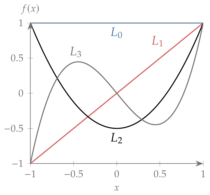
Figure 12.10:The first few Legendre polynomials.
From the Gaussian quadrature derivation, we find that we can integrate any polynomial of order exactly by choosing the node positions as the roots of the Legendre polynomial , with the corresponding weights given by
Legendre polynomials are defined over the interval , but we can reformulate them for an arbitrary interval through a change of variables:
where .
Using the change of variables, we can write
Now, applying a quadrature rule, we can approximate the integral as
where the node locations and respective weights come from the Legendre polynomials.
Recall that what we are after in this section is not just any generic integral but, rather, metrics such as the expected value,
As compared to our original integral (Equation 12.12), we have an additional function , referred to as a weight function. Thus, we extend the definition of orthogonal polynomials (Equation 12.17) to orthogonality with respect to the weight , also known as a weighted inner product:
For our purposes, the weight function is , or it is related to it through a change of variables.
Orthogonal polynomials for various weight functions are listed in Table 1. The weight function in the table does not always correspond exactly to the typically used PDF , so a change of variables (like Equation 12.22) might be needed. The formula described previously is known as Gauss–Legendre quadrature, whereas the variants listed in Table 1 are called Gauss–Hermite, and so on. Formulas and tables with node locations and corresponding weight values exist for most standard probability distributions. For any given weight function, we can generate orthogonal polynomials,7 and we can generate orthogonal polynomials for general distributions (e.g., ones that were empirically derived).
Table 1:Orthogonal polynomials that correspond to some common probability distributions.
| Prob. dist. | Weight function | Polynomial | Support range |
| Uniform | 1 | Legendre | |
| Normal | Hermite | ||
| Exponential | Laguerre | ||
| Beta | Jacobi | ||
| Gamma | Generalized Laguerre |
We now provide more details on Gauss–Hermite quadrature because normal distributions are common. The Hermite polynomials () follow the recurrence relationship,
where , and .
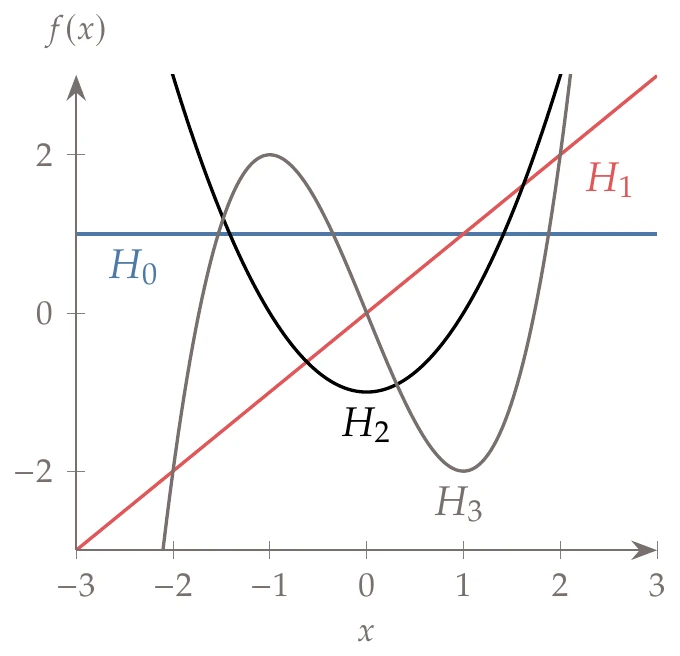
Figure 12.11:The first few Hermite polynomials.
The first few polynomials are plotted in Figure 12.11. For Gauss–Hermite quadrature, the nodes are positioned at the roots of , and their weights are
A coordinate transformation is needed because the standard normal distribution differs slightly from the weight function in Table 1. For example, if we are seeking an expected value, with normally distributed, then the integral is given by
We use the change of variables,
Then, the resulting integral becomes
This is now in the appropriate form, so the quadrature rule (using the Hermite nodes and weights) is
Gaussian quadrature does not naturally lead to nesting, which, as previously mentioned, can increase the accuracy by adding points to a given quadrature. However, methods such as Gauss–Konrod quadrature adapt Gaussian quadrature to utilize nesting. Although Gaussian quadrature is often used to compute one-dimensional integrals efficiently, it is not always the best method. For non-smooth functions, trapezoidal integration is usually preferable because polynomials are ill-suited for capturing discontinuities. Additionally, for periodic functions such as the one shown in Figure 12.4, the trapezoidal rule is better than Gaussian quadrature, exhibiting exponential convergence.89 This is most easily seen by using a Fourier series expansion.10
Clenshaw–Curtis quadrature applies this idea to a general function by employing a change of variables () to create a periodic function that can then be efficiently integrated with the trapezoidal rule. Clenshaw–Curtis quadrature also has the advantage that nesting is straightforward and thus desirable for higher-dimensional functions, as discussed next.
The direct quadrature methods discussed so far focused on integration in one dimension, but most problems have more than one random variable. Extending numerical integration to multiple dimensions (also known as cubature) is much more challenging. The most obvious extension for multidimensional quadrature is a full grid tensor product. This type of grid is created by discretizing each dimension and then evaluating at every combination of nodes. Mathematically, the quadrature formula can be written as
Although conceptually straightforward, this approach is subject to the curse of dimensionality.[7]The number of points we need to evaluate grows exponentially with the number of input dimensions.
One approach to dealing with exponential growth is to use a sparse grid method.11 The basic idea is to neglect higher-order cross terms. For example, assume that we have a two-dimensional problem and that both variables used a fifth-degree polynomial in the quadrature strategy. The cross terms would include terms up to the 10th order. Although we can integrate these high-order polynomials exactly, their contributions become negligible beyond a specific order. We specify a maximum degree that we want to include and remove all higher-order terms from the evaluation. This method significantly reduces the number of evaluation nodes, with minimal loss in accuracy.
For a problem with dimension and sample points in each dimension, the entire tensor grid has a computational complexity of . In contrast, the sparse grid method has a complexity of with comparable accuracy. This scaling alleviates the curse of dimensionality to some extent. However, the number of evaluation points is still strongly dependent on problem dimensionality, making it intractable in high dimensions.
12.3.3 Monte Carlo Simulation
Monte Carlo simulation is a sampling-based procedure that computes statistics and output distributions. Sampling methods approximate the integrals mentioned in the previous section by using the law of large numbers. The concept is that output probability distributions can be approximated by running the simulation many times with randomly sampled inputs from the corresponding probability distributions. There are three steps:
Random sampling. Sample points from the input probability distributions using a random number generator.
Numerical experimentation. Evaluate the outputs at these points, .
Statistical analysis. Compute statistics on the discrete output distribution .
For example, the discrete form of the mean is
and the unbiased estimate of the variance is computed as
We can also estimate by counting how many times the constraint was satisfied and dividing by . If we evaluate enough samples, our output statistics converge to the actual values by the law of large numbers. Therein also lies this method’s disadvantage: it requires a large number of samples.
Monte Carlo simulation has three main advantages. First, the convergence rate is independent of the number of inputs. Whether we have 3 or 300 random input variables, the convergence rate is similar because we randomize all input variables for each sample. This is an advantage over direct quadrature for high-dimensional problems because, unlike quadrature, Monte Carlo does not suffer from the curse of dimensionality. Second, the algorithm is easy to parallelize because all of the function evaluations are independent. Third, in addition to statistics like the mean and variance, Monte Carlo generates the output probability distributions. This is a unique advantage compared with first-order perturbation and direct quadrature, which provide summary statistics but not distributions.
The major disadvantage of the Monte Carlo method is that even though the convergence rate does not depend on the number of inputs, the convergence rate is slow—. This means that every additional digit of accuracy requires about 100 times more samples. It is also hard to know which value of to use a priori. Usually, we need to determine an appropriate value for through convergence testing (trying larger values until the statistics converge).
One approach to achieving converged statistics with fewer iterations is to use Latin hypercube sampling (LHS) or low-discrepancy sequences, as discussed in Section 10.2. Both methods allow us to approximate the input distributions with fewer samples. Low-discrepancy sequences are particularly well suited for this application because convergence testing is iterative. When combined with low-discrepancy sequences, the method is called quasi-Monte Carlo, and the scaling improves to . Thus, each additional digit of accuracy requires 10 times as many samples. Even with better sampling methods, many simulations are usually required, which can be prohibitive if used as part of an OUU problem.
12.3.4 Polynomial Chaos
Polynomial chaos (also known as spectral expansions) is a class of forward-propagation methods that take advantage of the inherent smoothness of the outputs of interest using polynomial approximations.[8]
The method extends the ideas of Gaussian quadrature to estimate the output function, from which the output distribution and other summary statistics can be efficiently generated. In addition to using orthogonal polynomials to evaluate integrals, we use them to approximate the output function. As in Gaussian quadrature, the polynomials are orthogonal with respect to a specified probability distribution (see Equation 12.25 and Table 1). A general function that depends on uncertain variables can be represented as a sum of basis functions (which are usually polynomials) with weights ,
In practice, we truncate the series after terms and use
The required number of terms for a given input dimension and polynomial order is
This approach amounts to a truncated generalized Fourier series.
By definition, we choose the first basis function to be . This means that the first term in the series is a constant (polynomial of order 0). Because the basis functions are orthogonal, we know that
Polynomial chaos consists of three main steps:
Select an orthogonal polynomial basis.
Compute coefficients to fit the desired function.
Compute statistics on the function of interest.
These three steps are described in the following sections. We begin with the last step because it provides insight for the first two.
Compute Statistics
Using the polynomial approximation (Equation 12.36) in the definition of the mean, we obtain
The coefficients are constants that can be taken out of the integral, so we can write
We can multiply all terms by without changing anything because , so we can rewrite this expression in terms of the inner product as
Because the polynomials are orthogonal, all the terms except the first are zero (see Equation 12.38). From the definition of a PDF (Equation A.63), we know that the first term is 1. Thus, the mean of the function is simply the zeroth coefficient,
We can derive a formula for the variance using a similar approach.
Substituting the polynomial representation (Equation 12.36) into the definition of variance and using the same techniques used in deriving the mean, we obtain
That last step is just the definition of the weighted inner product (Equation 12.25), providing the variance in terms of the coefficients and polynomials:
The inner product can often be computed analytically. For example, using Hermite polynomials with a normal distribution yields
For cases without analytic solutions, Gaussian quadrature of this inner product is still straightforward and exact because it only includes polynomials.
For multiple uncertain variables, the formulas are the same, but we use multidimensional basis polynomials. Denoting these multidimensional basis polynomials as , we can write
The multidimensional basis polynomials are defined by products of one-dimensional polynomials, as detailed in the next section. Polynomial chaos computes the mean and variance using these equations and our definition of the inner product. Other statistics can be estimated by sampling the polynomial expansion. Because we now have a simple polynomial representation that no longer requires evaluating the original (potentially expensive) function , we can use sampling procedures (e.g., Monte Carlo) to create output distributions without incurring high costs. Of course, we have to evaluate the function to generate the coefficients, as we will discuss later.
Selecting an Orthogonal Polynomial Basis
As discussed in Section 12.3.2, we already know appropriate orthogonal polynomials for many continuous probability distributions (see Table 1[9]). We also have methods to generate other exponentially convergent polynomial sets for any given empirical distribution.13
The multidimensional basis functions we need are defined by tensor products. For example, if we had two variables from a uniform probability distribution (and thus Legendre bases), then the polynomials up through the second-order terms would be as follows:
The term, for example, does not appear in this list because it is a third-order polynomial, and we truncated the series after the second-order terms. We should expect this number of basis functions because Equation 12.37 with and yields .
Determine Coefficients
Now that we have selected an orthogonal polynomial basis, , we need to determine the coefficients in Equation 12.36. We discuss two approaches for determining the coefficients. The first approach is quadrature, which is also known as spectral projection. The second is with regression, which is also known as stochastic collocation.
Let us start with the quadrature approach. Beginning with the polynomial approximation
we take the inner product of both sides with respect to ,
Using the orthogonality property of the basis functions (Equation 12.38), all the terms in the summation are zero except for
Thus, we can find each coefficient by
where we replaced the inner product with the definition given by Equation 12.17.
As expected, the zeroth coefficient corresponds to the definition of the mean,
These coefficients can be obtained through multidimensional quadrature (see Section 12.3.2) or Monte Carlo simulation (Section 12.3.3), which means that this approach inherits the same limitations of the chosen quadrature approach. However, the process can be more efficient if the selected basis functions are good approximations of the distributions. These integrals are usually evaluated using Gaussian quadrature (e.g., Gauss–Hermite quadrature if is a normal distribution).
Suppose all we are interested in is the mean (Equation 12.41 and Equation 12.51). In that case, the polynomial chaos approach amounts to just Gaussian quadrature. However, if we want to compute other statistical properties or produce an output PDF, the additional effort of obtaining the higher-order coefficients produces a polynomial approximation of that we can then sample to predict other quantities of interest.
It may appear that to estimate (Equation 12.36), we need to know (Equation 12.50). The distinction is that we just need to be able to evaluate at some predefined quadrature points, which in turn gives a polynomial approximation for any .
The second approach to determining the coefficients is regression. Equation 12.36 is linear, so we can estimate the coefficients using least squares (although an underdetermined system with regularization can be used as well). If we evaluate the function times, where is the sample, the resulting linear system is as follows:
As a rule of thumb, the number of sample points should be at least twice as large as the number of unknowns, . The sampling points, also known as the collocation points, typically correspond to the nodes in the corresponding quadrature strategy or utilize random sequences.[10]
12.4 Summary
Engineering problems are subject to variation under uncertainty. OUU deals with optimization problems where the design variables or other parameters have uncertain variability. Robust design optimization seeks designs that are less sensitive to inherent variability in the objective function. Common OUU objectives include minimizing the mean or standard deviation or performing multiobjective trade-offs between the mean performance and standard deviation. Reliable design optimization seeks designs with a reduced probability of failure, considering the variability in the constraint values. To quantify robustness and reliability, we need a forward-propagation procedure that propagates the probability distributions of the inputs (either design variables or parameters that are fixed during optimization) to the statistics or probability distributions of the outputs (objective and constraint functions). Four classes of forward propagation methods were discussed in this chapter.[11]Perturbation methods use a Taylor series expansion of the output functions to estimate the mean and variance. These methods can be efficient for a range of problem sizes, especially if accurate derivatives are available. Their main weaknesses are that they require derivatives (and hence second derivatives when using a gradient-based optimization), only work well with symmetric input probability distributions, and only provide the mean and variance (for first-order methods).
Direct quadrature uses numerical quadrature to evaluate the summary statistics. This process is straightforward and effective. Its primary weakness is that it is limited to low-dimensional problems (number of random inputs). Sparse grids enable these methods to handle a higher number of dimensions, but the scaling is still lacking.
Monte Carlo methods approximate the summary statistics and output distributions using random sampling and the law of large numbers. These methods are straightforward to use and are independent of the problem dimension. Their major weakness is that they are inefficient. However, because the alternatives are intractable for a large number of random inputs, Monte Carlo is an appropriate choice for many high-dimensional problems.
Polynomial chaos represents uncertain variables as a sum of orthogonal basis functions. This method is often a more efficient way to characterize both statistical moments and output distributions. However, the methodology is usually limited to a small number of dimensions because the number of required basis functions grows exponentially.
Problems
Although we maintain a distinction in this book, some of the literature includes both of these concepts under the umbrella of “robust optimization”.
Instead of using expected power directly, wind turbine designers use annual energy production, which is the expected power multiplied by utilization time.
Even characterizing input uncertainty might not be straightforward, but for forward propagation, we assume this information is provided.
This is the same issue as with the full factorial sampling used to construct surrogate models in Section 10.2.
Other polynomials can be used, but these polynomials are optimal because they yield exponential convergence.
This list is not exhaustive. For example, the methods discussed in this chapter are nonintrusive. Intrusive polynomial chaos uses expansions inside governing equations. Like intrusive methods for derivative computation (Chapter 6), intrusive methods for forward propagation require more implementation effort but are more accurate and efficient.
- Martins, J. R. R. A. (2020). Perspectives on aerodynamic design optimization. In Proceedings of the AIAA SciTech Forum. American Institute of Aeronautics. 10.2514/6.2020-0043
- Stanley, A. P. J., & Ning, A. (2019). Coupled wind turbine design and layout optimization with non-homogeneous wind turbines. Wind Energy Science, 4(1), 99–114. 10.5194/wes-4-99-2019
- Gagakuma, B., Stanley, A. P. J., & Ning, A. (2021). Reducing wind farm power variance from wind direction using wind farm layout optimization. Wind Engineering. 10.1177/0309524X20988288
- Padrón, A. S., Thomas, J., Stanley, A. P. J., Alonso, J. J., & Ning, A. (2019). Polynomial chaos to efficiently compute the annual energy production in wind farm layout optimization. Wind Energy Science, 4, 211–231. 10.5194/wes-4-211-2019
- Cacuci, D. (2003). Sensitivity & Uncertainty Analysis (Vol. 1). Chapman. 10.1201/9780203498798
- Parkinson, A., Sorensen, C., & Pourhassan, N. (1993). A general approach for robust optimal design. Journal of Mechanical Design, 115(1), 74. 10.1115/1.2919328
- Golub, G. H., & Welsch, J. H. (1969). Calculation of Gauss quadrature rules. Mathematics of Computation, 23(106), 221–230. 10.1090/S0025-5718-69-99647-1
- Wilhelmsen, D. R. (1978). Optimal quadrature for periodic analytic functions. SIAM Journal on Numerical Analysis, 15(2), 291–296. 10.1137/0715020
- Trefethen, L. N., & Weideman, J. A. C. (2014). The exponentially convergent trapezoidal rule. SIAM Review, 56(3), 385–458. 10.1137/130932132
- Johnson, S. G. (2010). Notes on the convergence of trapezoidal-rule quadrature. http://math.mit.edu/~stevenj/trapezoidal.pdf
- Smolyak, S. A. (1963). Quadrature and interpolation formulas for tensor products of certain classes of functions. In Proceedings of the USSR Academy of Sciences (Vol. 148, pp. 1042–1045). 10.3103/S1066369X10030084
- Wiener, N. (1938). The homogeneous chaos. American Journal of Mathematics, 60(4), 897. 10.2307/2371268
- Eldred, M., Webster, C., & Constantine, P. (2008). Evaluation of non-intrusive approaches for Wiener–Askey generalized polynomial chaos. In Proceedings of the 49th AIAA Structures, Structural Dynamics, and Materials Conference. American Institute of Aeronautics. 10.2514/6.2008-1892
- Adams, B. M., Bohnhoff, W. J., Dalbey, K. R., Ebeida, M. S., Eddy, J. P., Eldred, M. S., Hooper, R. W., Hough, P. D., Hu, K. T., Jakeman, J. D., Khalil, M., Maupin, K. A., Monschke, J. A., Ridgway, E. M., Rushdi, A. A., Seidl, D. T., Stephens, J. A., Swiler, L. P., & Winokur, J. G. (2021). Dakota, a multilevel parallel object-oriented framework for design optimization, parameter estimation, uncertainty quantification, and sensitivity analysis: Version 6.14 user’s manual [Sandia Technical Report]. Sandia National Laboratories. https://dakota.sandia.gov/content/manuals
- Feinberg, J., & Langtangen, H. P. (2015). Chaospy: An open source tool for designing methods of uncertainty quantification. Journal of Computational Science, 11, 46–57. 10.1016/j.jocs.2015.08.008