Appendix: Test Problems
D.1 Unconstrained Problems
D.1.1 Slanted Quadratic Function
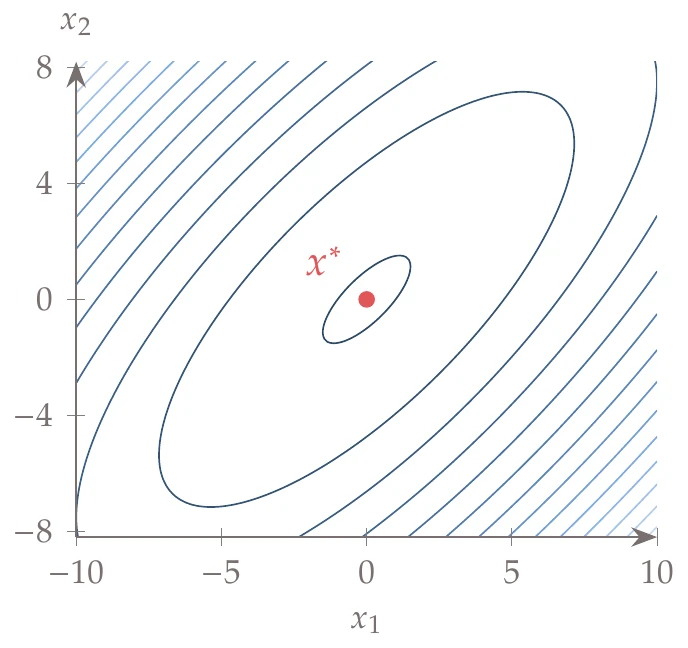
Figure D.1:Slanted quadratic function for .
This is a smooth two-dimensional function suitable for a first test of a gradient-based optimizer:
where . A value of zero corresponds to perfectly circular contours. As increases, the contours become increasingly slanted. For , the quadratic becomes semidefinite, and there is a line of weak minima. For , the quadratic is indefinite, and there is no minimum. An intermediate value of is suitable for first tests and yields the contours shown in Figure D.1.
Global minimum: at .
D.1.2 Rosenbrock Function
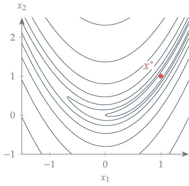
Figure D.2:Rosenbrock function.
The two-dimensional Rosenbrock function, shown in Figure D.2, is also known as Rosenbrock’s valley or banana function. This function was introduced by Rosenbrock,1 who used it as a benchmark problem for optimization algorithms.
The function is defined as follows:
This became a classic benchmarking function because of its narrow turning valley. The large difference between the maximum and minimum curvatures, and the fact that the principal curvature directions change along the valley, makes it a good test for quasi-Newton methods.
The Rosenbrock function can be extended to dimensions by defining the sum,
Global minimum: at .
Local minimum: For , a local minimum exists near .
D.1.3 Bean Function
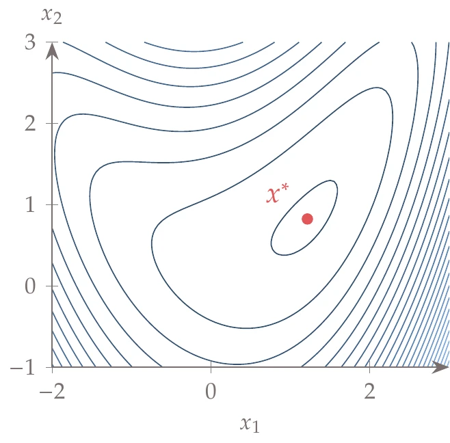
Figure D.3:Bean function.
The “bean” function was developed in this book as a milder version of the Rosenbrock function: it has the same curved valley as the Rosenbrock function but without the extreme variations in curvature. The function, shown in Figure D.3, is
Global minimum: at .
D.1.4 Jones Function
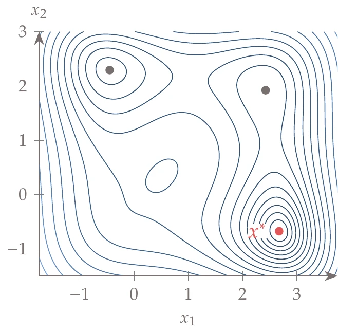
Figure D.4:Jones multimodal function.
This is a fourth-order smooth multimodal function that is useful to test global search algorithms and also gradient-based algorithms starting from different points. There are saddle points, maxima, and minima, with one global minimum. This function, shown in Figure D.4 along with the local and global minima, is
Global minimum: at .
Local minima: at .
at .
D.1.5 Hartmann Function
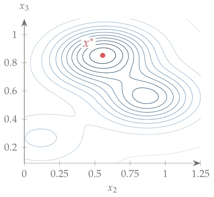
Figure D.5:An slice of Hartmann function at .
The Hartmann function is a three-dimensional smooth function with multiple local minima:
where
A slice of the function, at the optimal value of , is shown in Figure D.5.
Global minimum: at .
D.1.6 Aircraft Wing Design
We want to optimize the rectangular planform wing of a general aviation-sized aircraft by changing its wingspan and chord (see Example 1.1). In general, we would add many more design variables to a problem like this, but we are limiting it to a simple two-dimensional problem so that we can easily visualize the results.
The objective is to minimize the required power, thereby taking into account drag and propulsive efficiency, which are speed dependent. The following describes a basic performance estimation methodology for a low-speed aircraft. Implementing it may not seem like it has much to do with optimization. The physics is not important for our purposes, but practice translating equations and concepts into code is an important element of formulating optimization problems in general.
In level flight, the aircraft must generate enough lift to equal the required weight, so
We assume that the total weight consists of a fixed aircraft and payload weight and a component of the weight that depends on the wing area —that is,
The wing can produce a certain lift coefficient () and so we must make the wing area () large enough to produce sufficient lift. Using the definition of lift coefficient, the total lift can be computed as
where is the dynamic pressure and
If we use a rectangular wing, then the wing area can be computed from the wingspan () and the chord () as
The aircraft drag consists of two components: viscous drag and induced drag. The viscous drag can be approximated as
For a fully turbulent boundary layer, the skin friction coefficient, , can be approximated as
In this equation, the Reynolds number is based on the wing chord and is defined as follows:
where is the air density, and is the air dynamic viscosity.
The form factor, , accounts for the effects of pressure drag. The wetted area, , is the area over which the skin friction drag acts, which is a little more than twice the planform area. We will use
The induced drag is defined as
where is the Oswald efficiency factor. The total drag is the sum of induced and viscous drag, .
Our objective function, the power required by the motor for level flight, is
where is the propulsive efficiency. We assume that our electric propellers have a Gaussian efficiency curve (real efficiency curves are not Gaussian, but this is simple and will be sufficient for our purposes):
In this problem, the lift coefficient is provided. Therefore, to satisfy the lift requirement in Equation D.8, we need to compute the velocity using Equation D.11 and Equation D.10 as
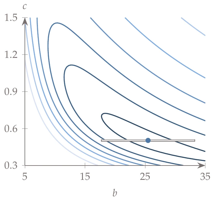
Figure D.6:Wing design problem with power requirement contour.
This is the same problem that was presented in Example 1.2 of Chapter 1. The optimal wingspan and chord are m and m, respectively, given the parameters. The contour and the optimal wing shape are shown in Figure D.6.
Because there are no structural considerations in this problem, the resulting wing has a higher wing aspect ratio than is realistic. This emphasizes the importance of carefully selecting the objective and including all relevant constraints.
The parameters for this problem are given as follows:
| Parameter | Value | Unit | Description |
| 1.2 | kg/m | Density of air | |
| kg/(m sec) | Viscosity of air | ||
| 1.2 | Form factor | ||
| 0.4 | Lift coefficient | ||
| 0.80 | Oswald efficiency factor | ||
| 1,000 | N | Fixed aircraft weight | |
| 8.0 | N/m | Wing area dependent weight | |
| 0.8 | Peak propulsive efficiency | ||
| 20.0 | m/s | Flight speed at peak propulsive efficiency | |
| 5.0 | m/s | Standard deviation of efficiency function |
D.1.7 Brachistochrone Problem
The brachistochrone problem is a classic problem proposed by Johann Bernoulli (see Section 2.2 for the historical background). Although this was originally solved analytically, we discretize the model and solve the problem using numerical optimization. This is a useful problem for benchmarking because you can change the number of dimensions.
A bead is set on a wire that defines a path that we can shape. The bead starts at some -position with zero velocity. For convenience, we define the starting point at .
From the law of conservation of energy, we can then find the velocity of the bead at any other location. The initial potential energy is converted to kinetic energy, potential energy, and dissipative work from friction acting along the path length, yielding the following:
Now that we know the speed of the bead as a function of , we can compute the time it takes to traverse an differential element of length :
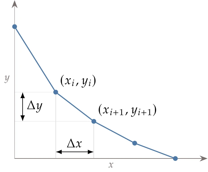
Figure D.7:A discretized representation of the brachistochrone problem.
To discretize this problem, we can divide the path into linear segments. As an example, Figure D.7 shows the wire divided into four linear segments (five nodes) as an approximation of a continuous wire. The slope is then a constant along a given segment, and . Making these substitutions results in
Performing the integration and simplifying (many steps omitted here) results in
where , and . The objective of the optimization is to minimize the total travel time, so we need to sum up the travel time across all of our linear segments:
Minimization is unaffected by multiplying by a constant, so we can remove the multiplicative constant for simplicity (we see that the magnitude of the acceleration of gravity has no effect on the optimal path):
The design variables are the positions of the path parameterized by . The endpoints must be fixed; otherwise, the problem is ill-defined, which is why there are design variables instead of . Note that is a parameter, meaning that it is fixed. We could space the any reasonable way and still find the same underlying optimal curve, but it is easiest to just use uniform spacing. As the dimensionality of the problem increases, the solution becomes more challenging. We will use the following specifications:
Starting point: m.
Ending point: m.
Kinetic coefficient of friction
The analytic solution for the case with friction is more difficult to derive, but the analytic solution for the frictionless case () with our starting and ending points is as follows:
where and .
D.1.8 Spring System
Consider a connected spring system of two springs with lengths of and and stiffnesses of and , fixed at the walls as shown in Figure D.8. An object with mass is suspended between the two springs. It will naturally deform such that the sum of the gravitational and spring potential energy, , is at the minimum.
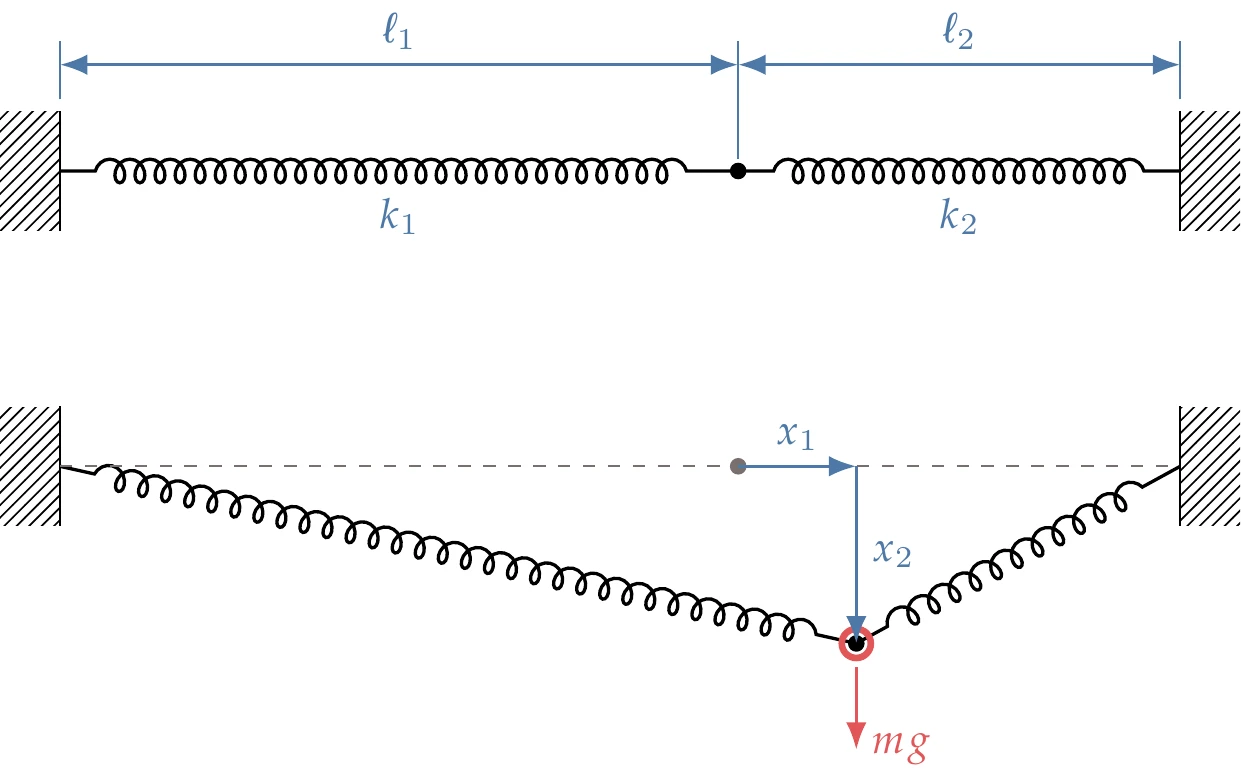
Figure D.8:Two-spring system with no applied force (top) and with applied force (bottom).
The total potential energy of the spring system is
where and are the changes in length for the two springs. With respect to the original lengths, and displacements and as shown, they are defined as
This can be minimized to determine the final location of the object.
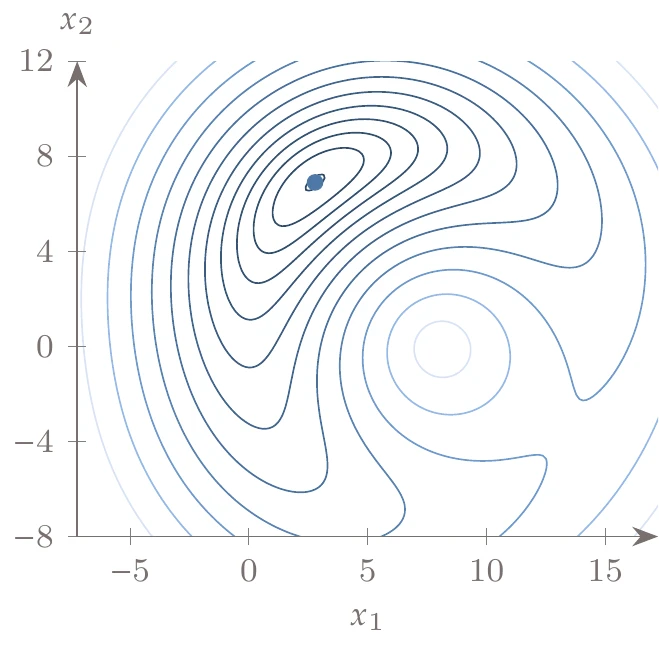
Figure D.9:Total potential energy contours for two-spring system.
With initial lengths of cm, cm; spring stiffnesses of Ncm, Ncm; and a force due to gravity of , the minimum potential energy is at . The contour of with respect to and is shown in Figure D.9.
The analytic derivatives can also be computed for use in a gradient-based optimization. The derivative of with respect to is
where the partial derivatives of and are
By letting and , the partial derivative of with respect to can be written as
Similarly, the partial derivative of with respect to can be written as
D.2 Constrained Problems
D.2.1 Barnes Problem
The Barnes problem was devised in a master’s thesis2 and has been used in various optimization demonstration studies. It is a good starter problem because it only has two dimensions for easy visualization while also including constraints.
The objective function contains the following coefficients:
| = 75.196 | = -3.8112 |
| = 0.12694 | = |
| = | = -6.8306 |
| = 0.030234 | = |
| = | = |
| = 0.25645 | = |
| = | = -28.106 |
| = | = |
| = | = |
| = | = -2.8673 |
| = 0.0005 |
For convenience, we define the following quantities:
The objective function is then:
There are three constraints of the form :
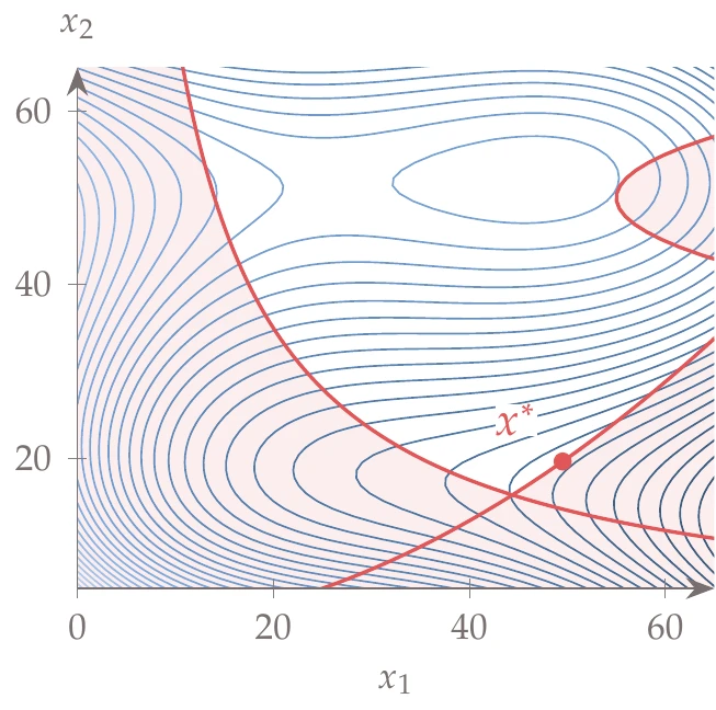
Figure D.10:Barnes function.
The problem also has bound constraints. The original formulation is bounded from in both dimensions, in which case the global optimum occurs in the corner at , with a local minimum in the middle. However, for our usage, we preferred the global optimum not to be in the corner and so set the bounds to in both dimensions. The contour of this function is plotted in Figure D.10.
Global minimum: at .
Local minimum: at .
D.2.2 Ten-Bar Truss
The 10-bar truss is a classic optimization problem.3 In this problem, we want to find the optimal cross-sectional areas for the 10-bar truss shown in Figure D.11. A simple truss finite-element code set up for this particular configuration is available in the book code repository.
The function takes in an array of cross-sectional areas and returns the total mass and an array of stresses for each truss member.
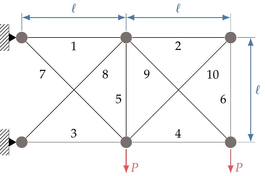
Figure D.11:Ten-bar truss and element numbers.
The objective of the optimization is to minimize the mass of the structure, subject to the constraints that every segment does not yield in compression or tension. The yield stress of all elements is psi, except for member 9, which uses a stronger alloy with a yield stress of psi. Mathematically, the constraint is
where the absolute value is needed to handle tension and compression (with the same yield strength for tension and compression). Absolute values are not differentiable at zero and should be avoided in gradient-based optimization if possible. Thus, we should put this in a mathematically equivalent form that avoids absolute value.
Each element should have a cross-sectional area of at least 0.1 in for manufacturing reasons (bound constraint). When solving this optimization problem, you may need to scale the objective and constraints.
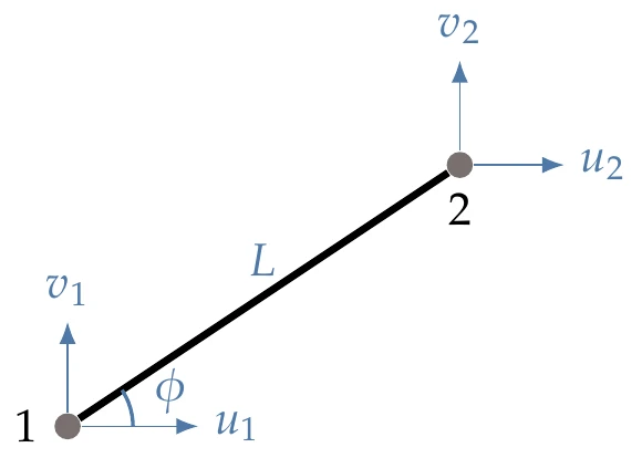
Figure D.12:A truss element oriented at some angle , where is measured from a horizontal line emanating from the first node, oriented in the positive direction.
Although not needed to solve the problem, an overview of the equations is provided. A truss element is the simplest type of structural finite element and only has an axial degree of freedom. The theory and derivation for truss elements are simple, but for our purposes, we skip to the result. Given a two-dimensional element oriented arbitrarily in space (Figure D.12), we can relate the displacements at the nodes to the forces at the nodes through a stiffness relationship.
In matrix form, the equation for a given element is . In detail, the equation is
where the displacement vector is . The meanings of the variables in the equation are described in Table 1.
Table 1:The variables used in the stiffness equation.
| Variable | Description |
| Force in the -direction at node | |
| Force in the -direction at node | |
| Modulus of elasticity of truss element material | |
| Area of truss element cross section | |
| Length of truss element | |
| Displacement in the -direction at node | |
| Displacement in the -direction at node |
The stress in the truss element can be computed from the equation , where is a scalar, is the same vector as before, and the element matrix (really a row vector because stress is one-dimensional for truss elements) is
The global structure (an assembly of multiple finite elements) has the same equations, and , but now contains displacements for all of the nodes in the structure, . If we have nodes and elements, then and are -vectors, is a matrix, is an matrix, and is an -vector. The elemental stiffness and stress matrices are first computed and then assembled into the global matrices. This is straightforward because the displacements and forces of the individual elements add linearly.
After we assemble the global matrices, we must remove any degrees of freedom that are structurally rigid (already known to have zero displacement). Otherwise, the problem is ill-defined, and the stiffness matrix will be ill-conditioned.
Given the geometry, materials, and external loading, we can populate the stiffness matrix and force vector. We can then solve for the unknown displacements from
With the solved displacements, we can compute the stress in each element using
- Rosenbrock, H. H. (1960). An automatic method for finding the greatest or least value of a function. The Computer Journal, 3(3), 175–184. 10.1093/comjnl/3.3.175
- Barnes, G. K. (1967). A comparative study of nonlinear optimization codes [Mathesis]. University of Texas at Austin.
- Venkayya, V. B. (1971). Design of optimum structures. Computers & Structures, 1(1–2), 265–309. 10.1016/0045-7949(71)90013-7